Managing your finances can be a hassle, especially when it comes to keeping track of your expenses. But it doesn't necessarily have to be, with tools like Google Sheets allowing you to easily create spending trackers for your monthly expenditure. While Google Sheets has several readymade templates you can use for this purpose, you can also create a custom monthly spending tracker from scratch.
Step 1: Consider what you want to include in your spending tracker
Before you start creating your spending tracker, you need to think about what things you want to include in it. It is a good idea to keep things simple, which will make visualizing and tracking expenses easier.
- Visit the Google Sheets webpage using your web browser and sign in to your Google account.
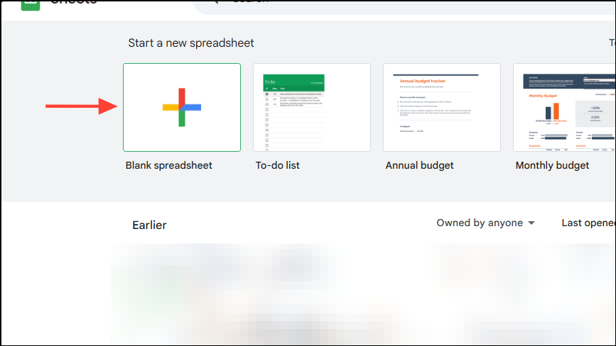
- Click on the 'Blank spreadsheet' option to create a new spreadsheet.
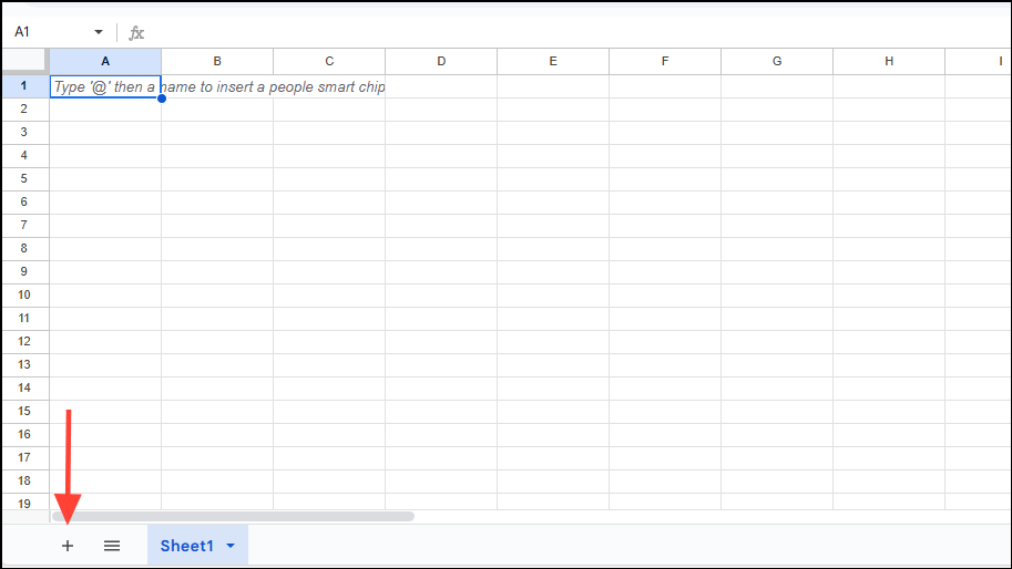
- When a new spreadsheet opens, click on the '+' button on the bottom left to create another sheet, since you will need two sheets for your expense manager. The first one will contain all your expense data while the second one will help you summarize and visualize it.
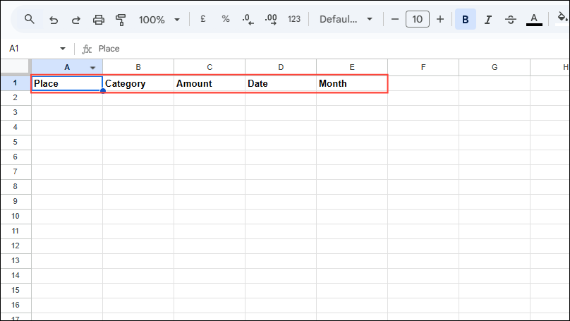
- Once both sheets are created, go to the first sheet and create five columns. Give them the following names:
- Place - the store from which you made your purchases.
- Category - the type of items you purchased.
- Amount - the amount of money you paid for that item.
- Date - the date on which you purchased the item.
- Month - the month in which you purchased the item.
Step 2: Create a menu for different spending categories
You will need to assign categories to transactions you enter in your expense tracker spreadsheet so you don't have to manually type them each time.
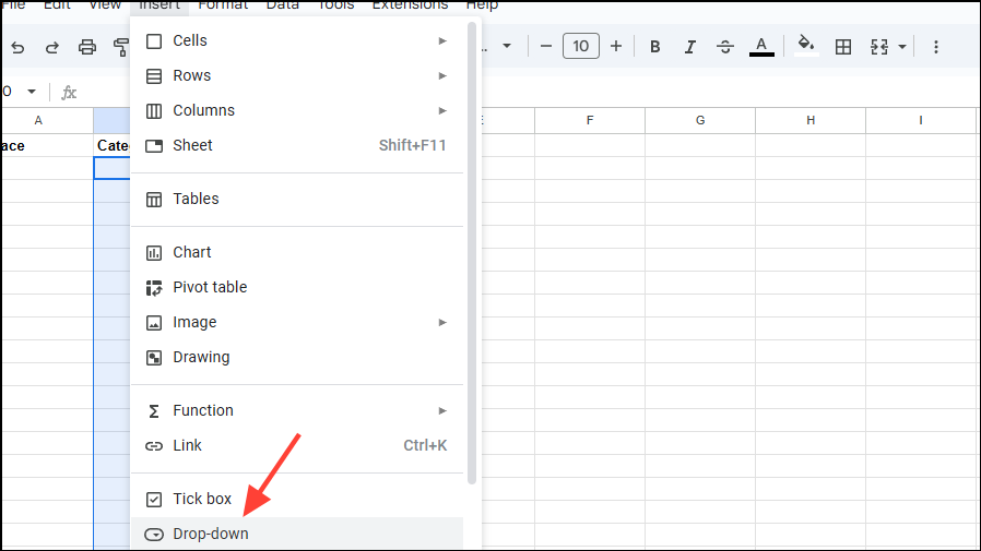
- Click on the 'Category' column and then press and hold the
CtrlorCMDkey depending on your machine before deselecting the title cell. Then click on the 'Insert' menu at the top.
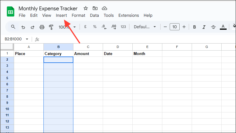
- Then select 'Drop-down' from the menu.
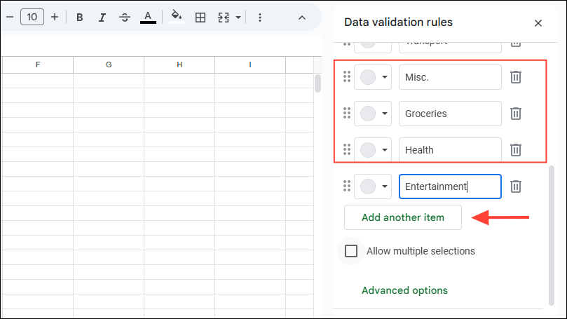
- A sidebar will open on the right. Now you can add the categories you wish to see in the expense tracker. Click on 'Add another item' to add more categories.
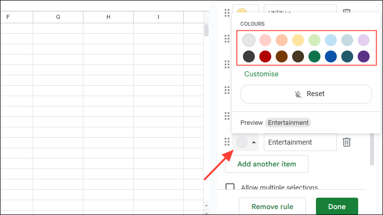
- Click on dropdown menus to the left of the categories you have added to color code them. Once you're finished, click on the 'Done' button at the bottom.
Step 3: Format your expense tracker
You will have to format your monthly expense tracker properly to ensure the currency and date formatting in each cell is consistent.
- To format your 'Date' column, click on the column heading to select the column.
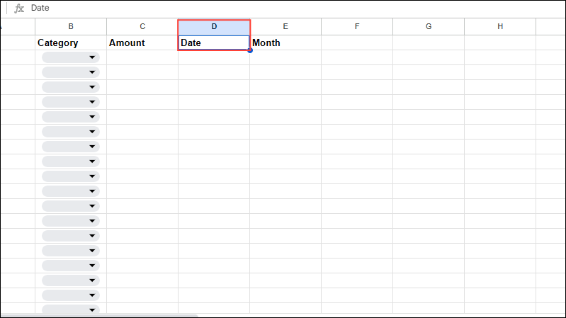
- Then click on the 'More Formats' option in the toolbar. It will will have the '123' symbol.
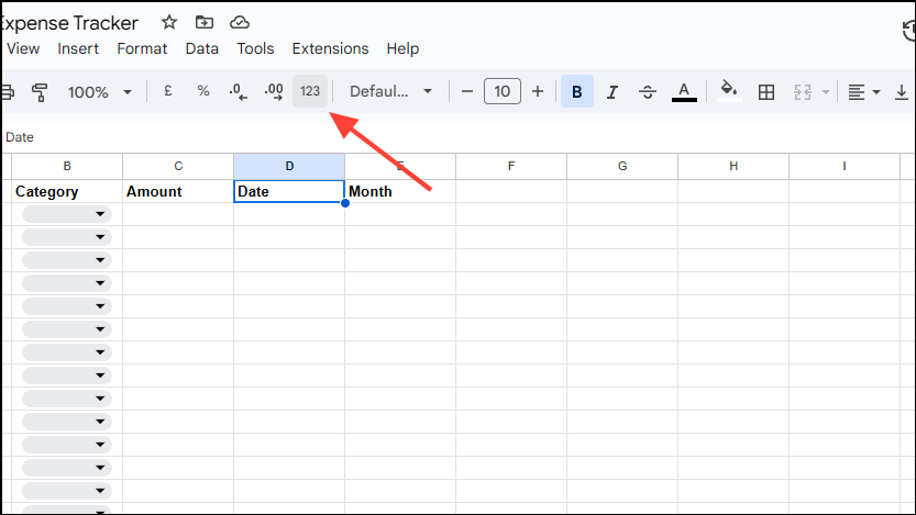
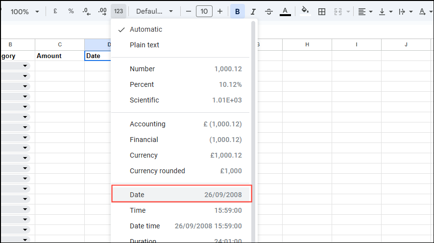
- Select 'Date' from the dropdown menu that appears on your screen.
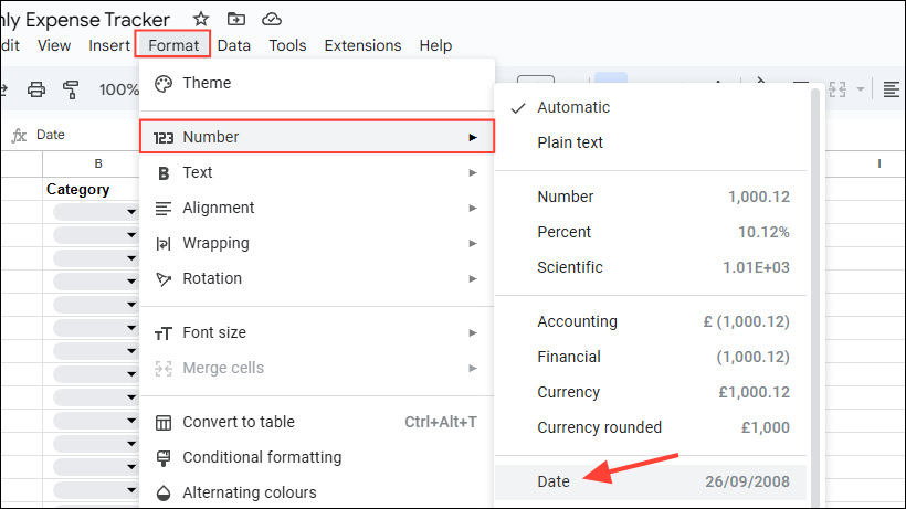
- An alternative method is to click on the 'Format' menu at the top and then go to 'Number' before selecting the 'Date' option.
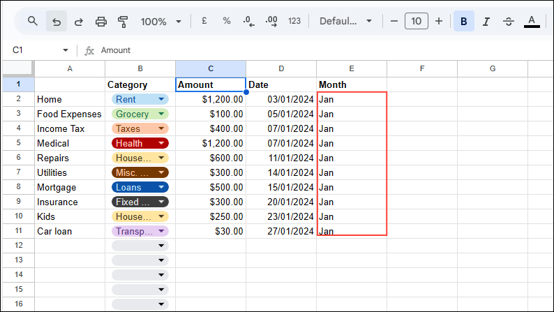
- The TEXT function lets you add month formatting to your spreadsheet and automatically shows the month of purchase by extracting information from the date.
To use it, you will have to click on the first row in the 'Month' column and use the following formula:=TEXT(cell reference of cell containing corresponding date,"mmm"). For instance, if the date is in Cell D2, type=TEXT(D2, "mmm")and you will automatically see the Month in the Month column.
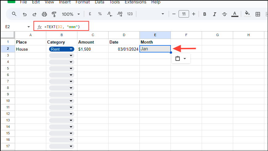
- Once you've filled in the rest of the columns, like Place, Category, Amount, and Date, you can click and drag the first cell in the Month column down to automatically fill the rest of the cells.
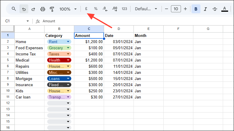
- You can also add currency formatting by clicking on the heading of the Amount column and then clicking on the
$or€symbol, whichever appears on the toolbar. If you cannot directly find it on the toolbar, click on the 'More formats' (123) option to access it. Make sure to enter the amounts in simple numbers before you add the currency formatting and Google Sheets will automatically add the currency symbol needed; otherwise, you'll run into unexpected errors.
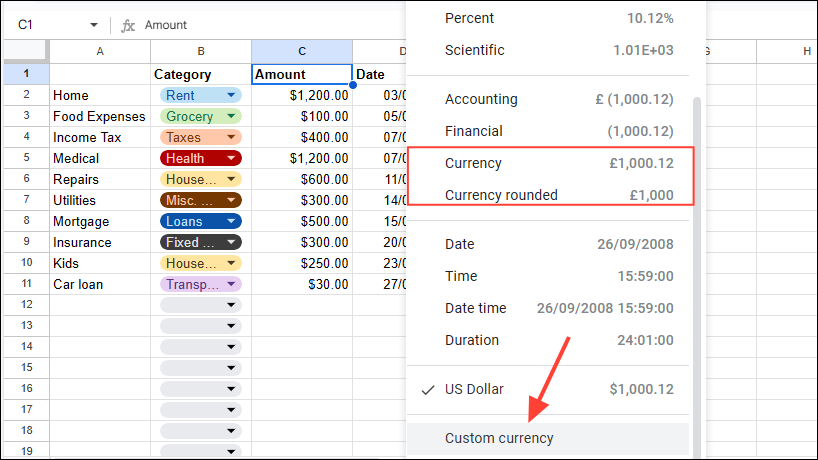
- In the 'More formats' menu, you can then choose between 'Currency', 'Currency rounded', and 'Custom currency'. You can select how the symbol and decimal points appear or choose a different currency. Pay attention to the currency symbol set by default, such as Dollar or Euro, and select the Custom currency accordingly, otherwise, you will get an error when using formulas.
Step 4: Use functions to create a summary of your expenses
- Once you've added the details of your expenses in your first spreadsheet, switch to the second sheet by clicking on its name at the bottom left.
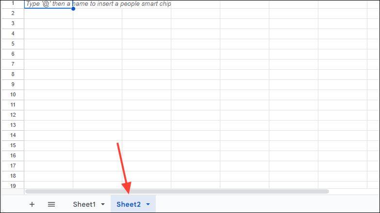
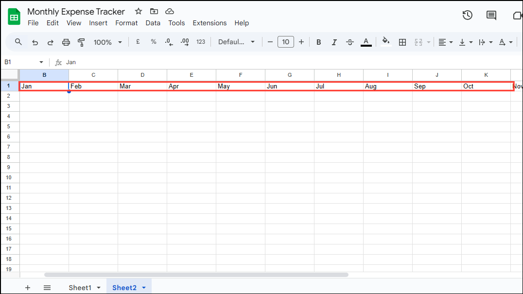
- Now, enter the first three letters of each month from cells B1 to M1. The category total shall appear in Cell N.
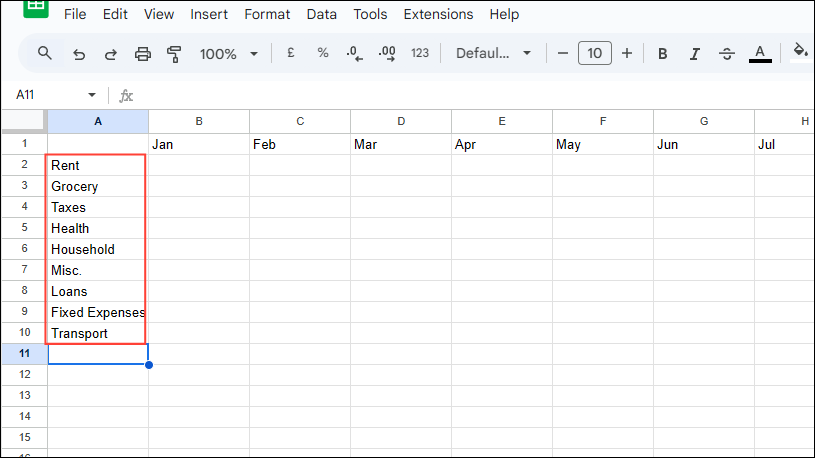
- Then enter the expense categories from the second cell of column A. These categories should correspond with the ones you've included in the first spreadsheet in the drop-down menu.
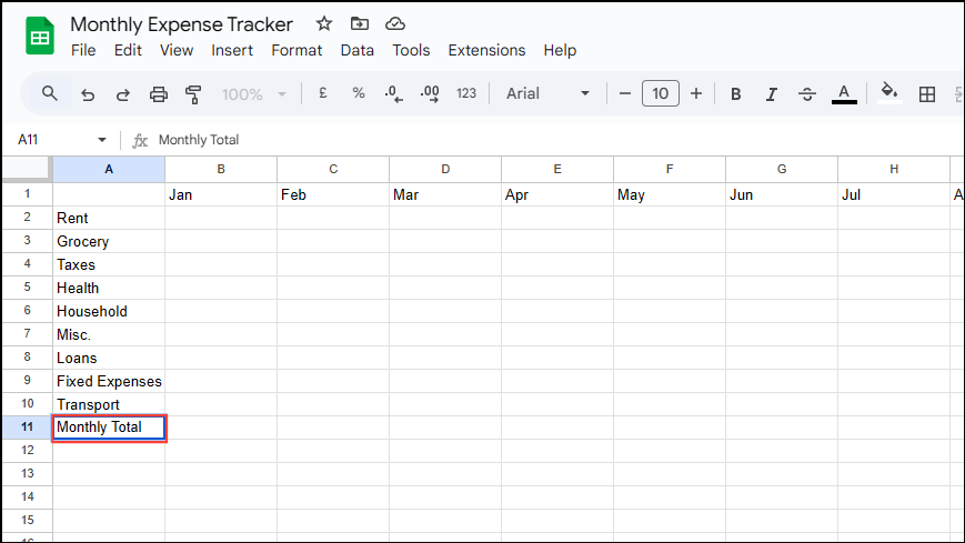
- In the row below the last category in the same column (column A), add the label 'Monthly Total'.
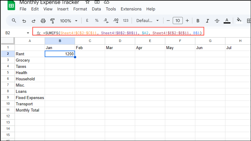
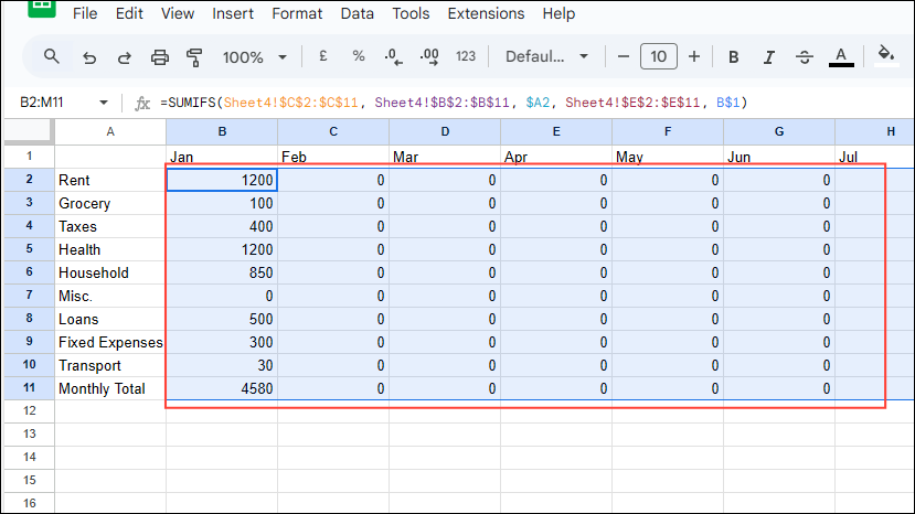
- To generate the expense summary, you need to use the SUMIFs formula. In Cell B2, you need to enter the formula:
=SUMIFS(Sheet1!$C$2:$C$11, Sheet1!$B$2:$B$11, $A2, Sheet1!$E$2:$E$11, B$1). Keep in mind that you will need to replace the name of the sheet, such as Sheet 1 in this case, with the sheet that contains your data and cell values with the ones corresponding to your sheet.
- Once you've entered the formula, click on cell B2 and drag it to the cell at the end next to the Monthly Total. Then drag it to the right till it reaches column M.
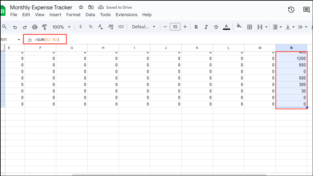
- Click on Column N2 and type
=SUM(B2:M2)before dragging it down to calculate the category total.
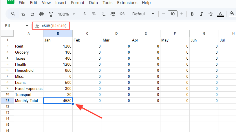
- You will also need to use the SUM function in the Monthly Total row to sum up the expenses of all categories in one month. Click on the cell on the right of the Monthly Total and use the formula
=SUM (B2:B10)or whatever the respective cells are in your sheet are, to sum up the values.
Step 5: Use sparklines and pie charts to visualize expenses
Google Sheets can also help you visualize your expenses using sparklines and pie charts.
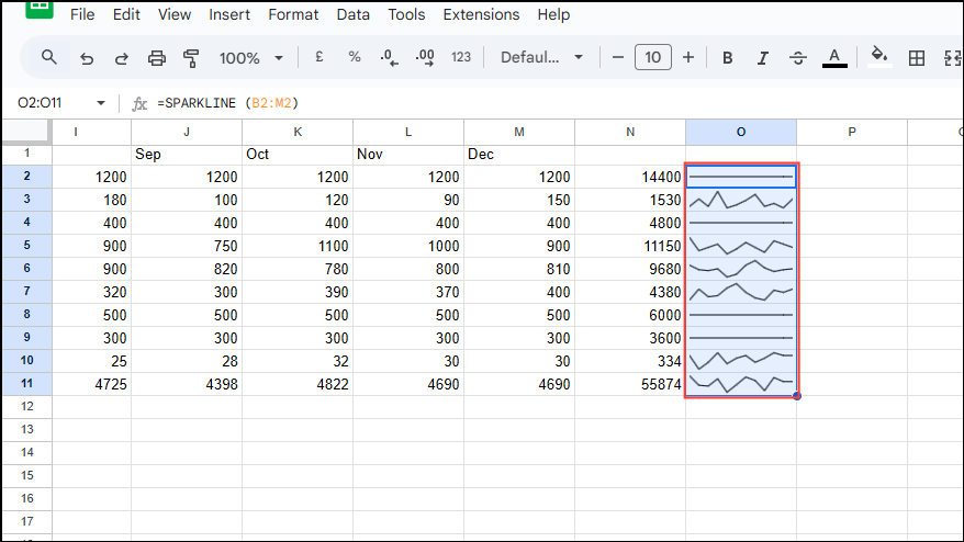
- Click on cell O2 and use the SPARKLINE formula by typing
=SPARKLINE(B2:M2).
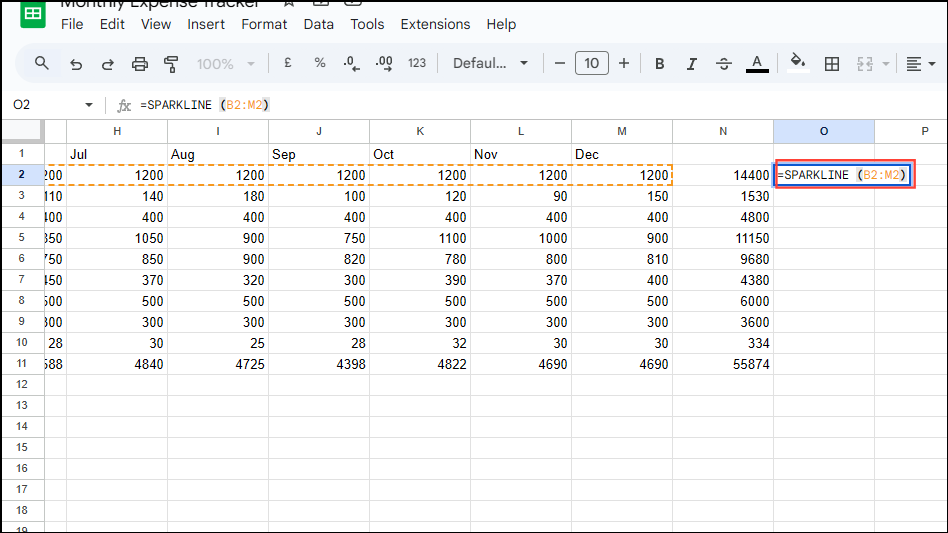
- You will get the sparkline for that particular category. Now drag it down to the last category and you will see the sparklines for all categories.
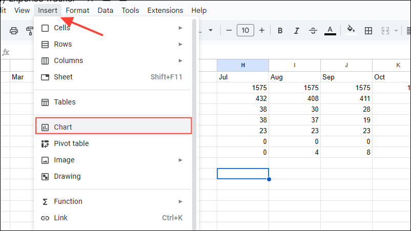
- Now, click on the 'Insert' menu and select 'Chart'.
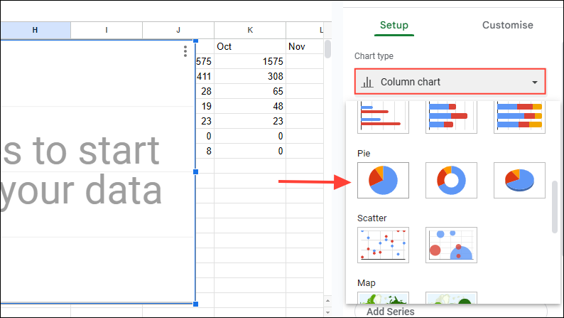
- Under the 'Chart type' dropdown menu, scroll down and select Pie chart.
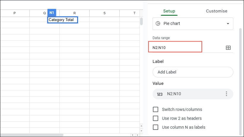
- In the 'Data range' section, type the range between your first and last cells in the Total column, for instance
N2:N10.
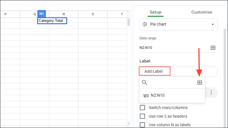
- Now click on the 'Add label' option and the icon with four squares so you can select a data range for your labels.
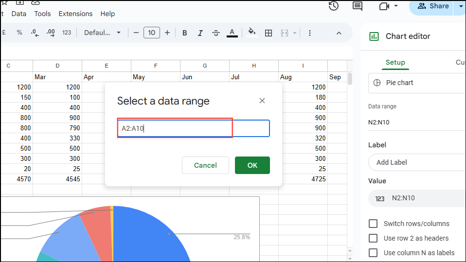
- Type in the data range, such as
A2:A10or whatever your data range for the labels is.
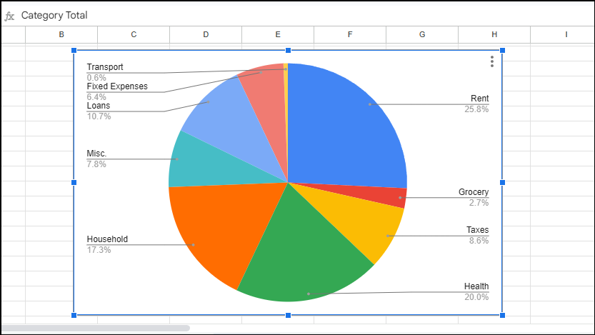
- The pie chart will show you all your expenses, breaking each of them down separately.
Step 6: View spending categories using filters
You can use filters to hide or sort transactions.
- Click on the column in your spreadsheet for which you want to sort your transactions.
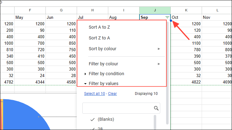
- Then click on the 'Create a filter' button on the toolbar, which will appear as an inverted triangle next to the 'Insert chart' button.
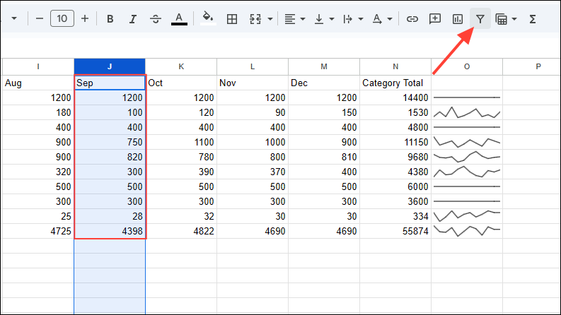
- Three lines will appear next to the column heading. Click on them and you will see various options. You can choose 'Filter by values', 'Sort A to Z', or other options to sort your expenses as you want. Then click on the 'OK' button to apply the changes.
Things to know
- Once you've created your expense tracker, it will automatically update itself when you add new expenses and show their breakdown in the pie chart.
- You can also convert the entries in the first sheet into a table if you find that doing so will make it easier to view and analyze your expenses.
- The biggest advantage of creating your own expense tracker rather than using a readymade template is that you can easily fix your spreadsheet if there is a problem with it.
- You can also install the Google Sheets app on your smartphone, which will make it easier to enter your expenses as and when they occur.

