
Microsoft Excel offers several tools and features for manipulating data, and Power Query is one of the best ones. This business analysis tool lets you import data from various sources and transform and manipulate it easily in Excel as needed. Basically, it eliminates repetitive tasks and can help reduce effort and save time.
A major advantage of Power Query is that you do not require any coding expertise or knowledge to use it. Let’s look at how you can use it to manipulate data in Microsoft Excel.
Accessing Power Query
Power Query is available in all versions of Microsoft Excel, starting with Excel 2010. From Excel 2016, it has been baked into the application directly.
In Excel 2016 And Later
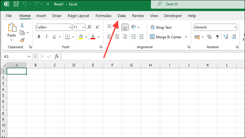
- Launch a new Excel worksheet and click the ‘Data’ tab on the menu bar.
- From the options in the ‘Data’ tab, click the ‘Get Data’ option on the upper left side below the menu bar.
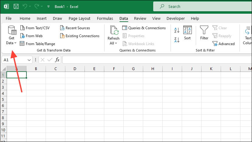
- This contains all the Power Query tools and options for importing and transforming data.
In Excel 2013 And 2010
For Excel versions 2013 and 2010, Power Query is available as a free add-on that you can download from the Microsoft website.
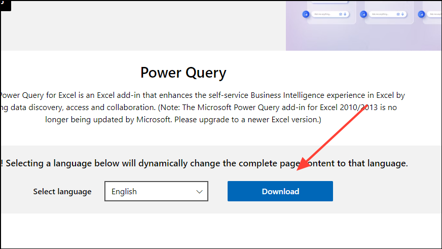
- Go to the Power Query download page and click the ‘Download’ button to start downloading the tool.
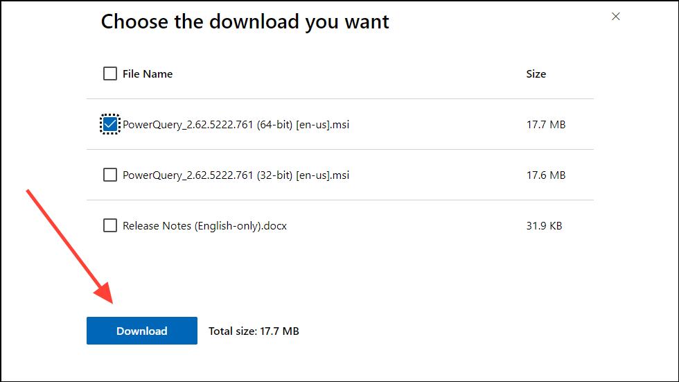
- When you click the ‘Download’ button, you will see a few options from which you can select the appropriate one depending on your system.
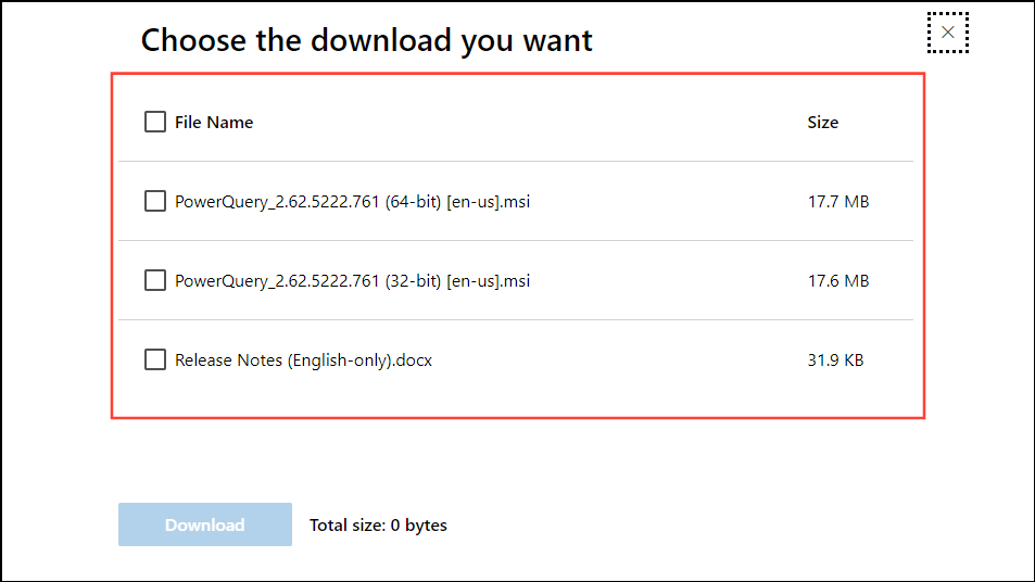
- After selecting the right option, click the ‘Download’ button to download the tool.
Using The Power Query Tool
With an Excel worksheet open, you can access the Power Query tool from the ‘Data’ tab and then the ‘Get Data’ option.
Importing Data
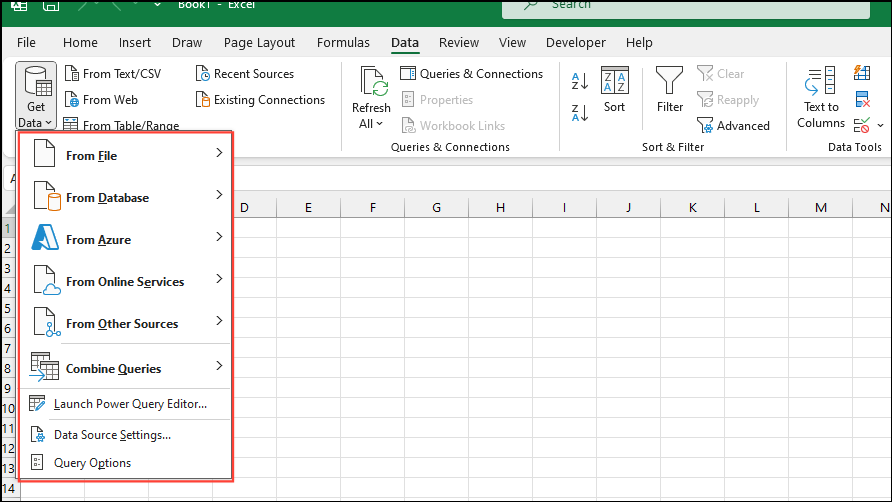
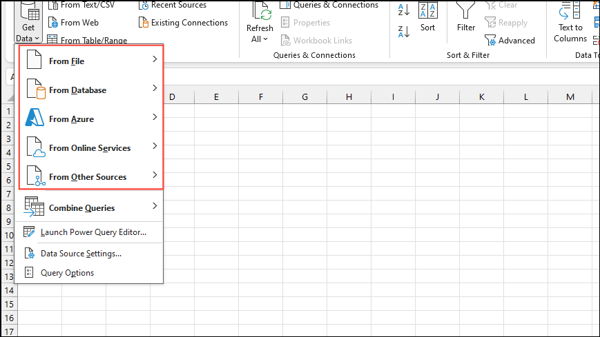
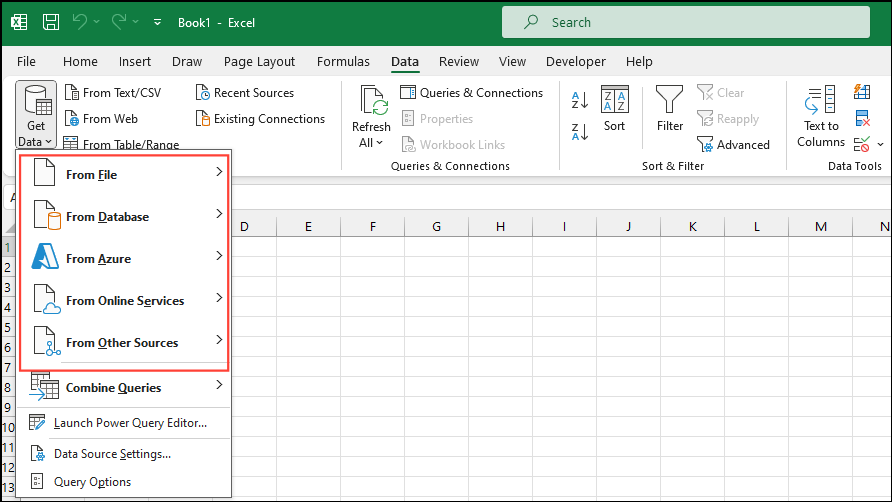
- When you click the ‘Get Data’ option, it will show the various sources from where you can import data. These include Excel workbooks, text or CSV files, XML, and JSON files.
Besides these, you can import data from online databases like SQL Server and Microsoft Access, among others. Other sources from which you can import data include Microsoft Azure and online services, like Salesforce and Facebook. - To import data, click on any of the options, such as ‘From File’, ‘From Database’, ‘From Azure’, ‘From Online Services’, and ‘From Other Sources’.
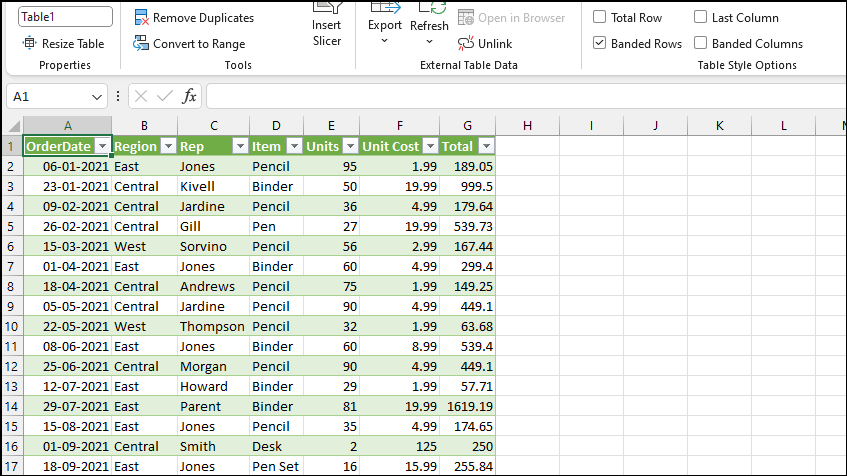
- When you import data, Excel will show you a pop-up displaying a preview of the data that will be loaded. Click the ‘Load’ button at the bottom to finish importing the data.
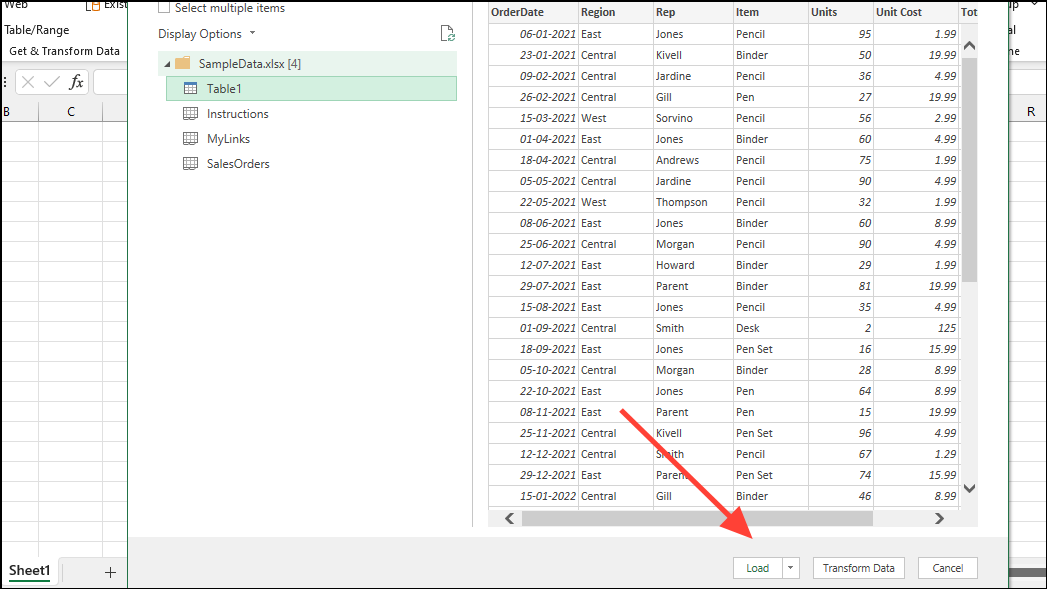
- Now you will see the data in your Excel worksheet and can apply different transformations to it.
Components of the Power Query Editor
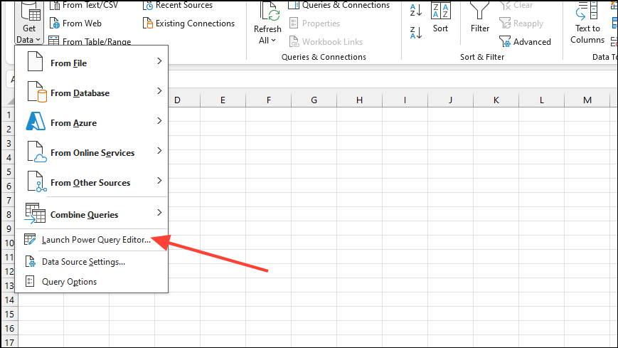
- You need the Power Query Editor to transform imported data as needed. Click the ‘Launch Power Query Editor’ after clicking the ‘Get Data’ button.
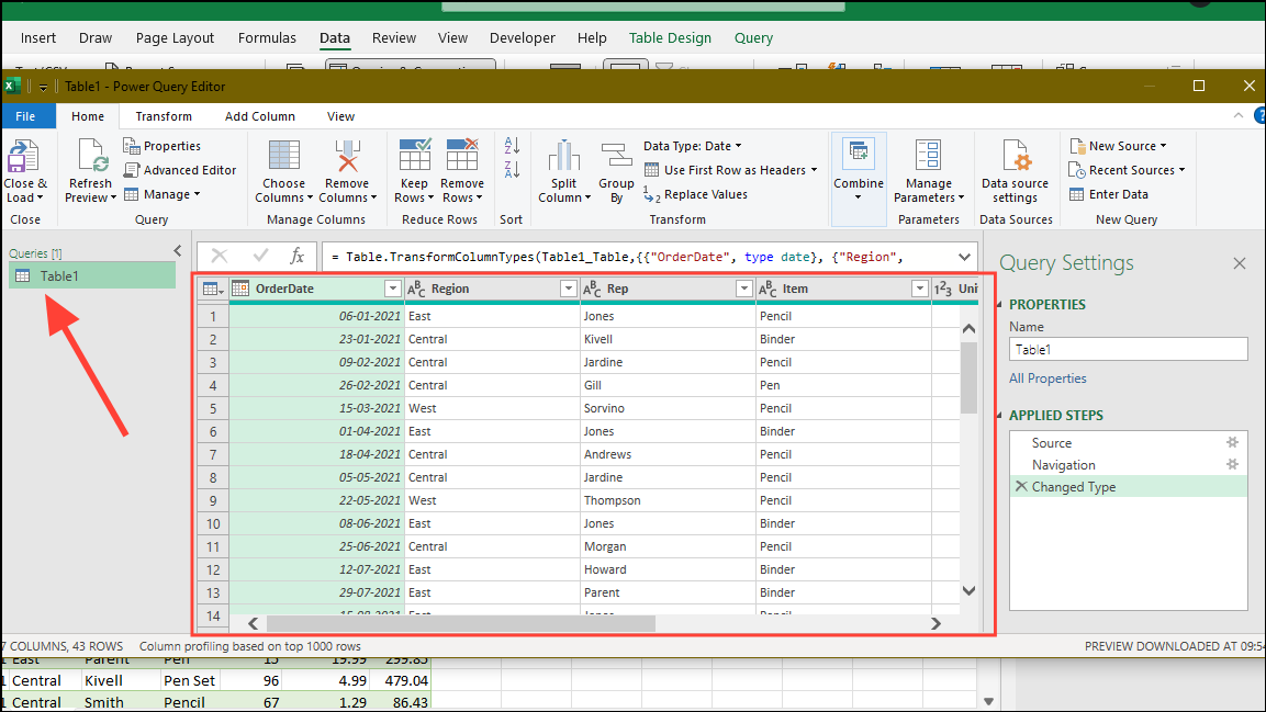
- This will launch the ‘Power Query Editor’, which is comprised of six main components. At the top, you will find the ‘Query Editor Ribbon’, which contains various commands under different tabs.
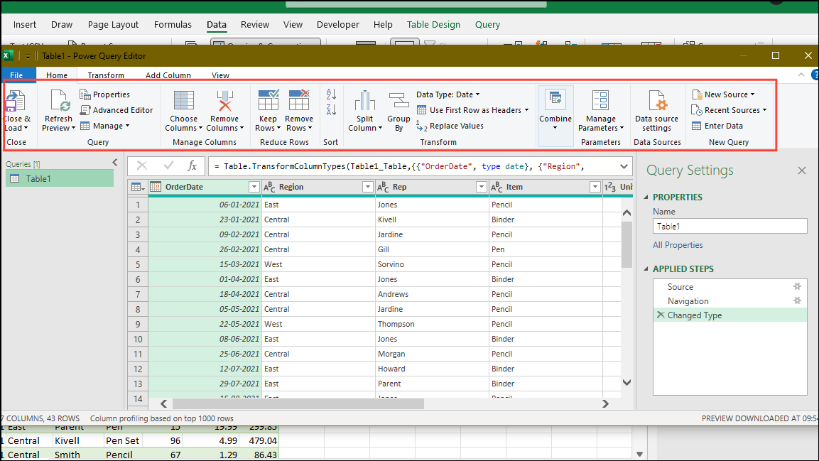
- Below the ‘Query Editor Ribbon’ on the left side is the ‘Query List’, which shows all the queries in the workbook. There will also be a ‘Data Preview’ section in the center, which shows all the transformations applied to the data.
- The ‘Formula Bar’ allows editing the M code of the transformation step. All transformations are recorded and appear as steps in the ‘Applied Steps’ area.
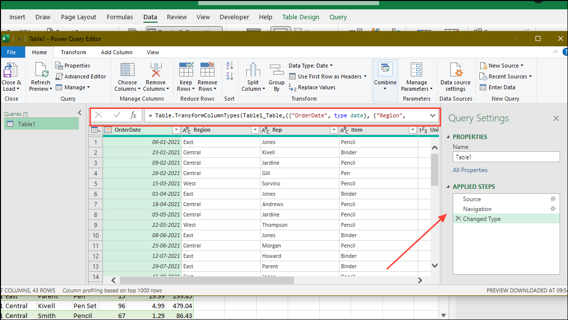
- The ‘Properties’ section allows you to provide queries with names.
Applying Transformations
You can apply various transformations to the data imported in the Power Query Editor. These include text formations, trimming, transposing, and more.
Text Transformations
Text can be transformed into upper or lower-case after you have imported it into the Editor.
- In the Power Query Editor, go to the ‘Transform’ tab at the top, and you will see several options, like ‘Transpose’, ‘Replace Values’, etc.
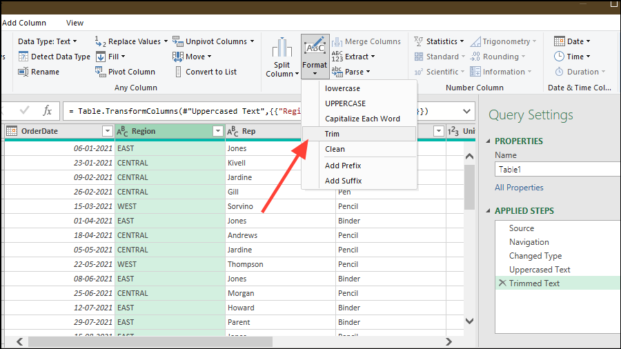
- The ‘Format’ option is present in the center, next to the ‘Split Column’ option. Click on it to view the available formatting options.
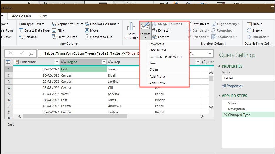
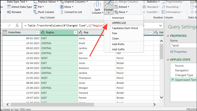
- Click on any option, such as ‘lowercase’ or ‘UPPERCASE’, to transform the text in the selected column into lowercase or uppercase. Similarly, clicking on other options will transform the text accordingly.
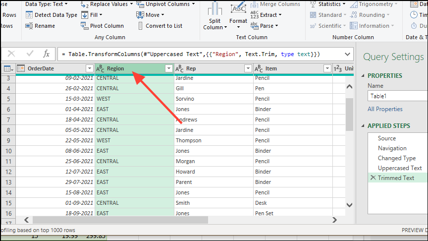
- The ‘Format’ option also allows you to remove all the white spaces by using the ‘Trim’ option. When you click the ‘Trim’ button, it will remove all extra white spaces from the text.
Splitting Columns
Apart from transforming the text, the Power Query Editor allows splitting columns in various ways.
- Once you have imported the data into the Power Query Editor, click on the column heading to select the entire column.
- Then click the ‘Split Column’ button to the left of the ‘Format’ button. This will give you a list of options that allow splitting the selected column in different ways.
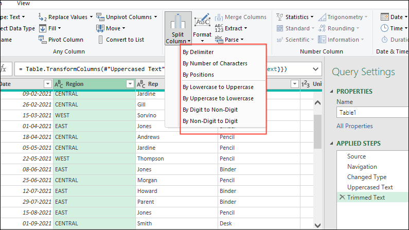
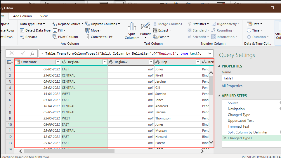
- To split the column by delimiter, click the respective option. This will show the split by delimiter pop-up, where you can select the delimiter, such as comma, colon, equals sign, etc.
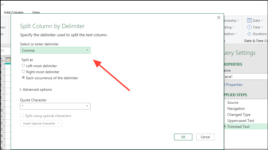
- Click the ‘OK’ button to split the column as desired, and you will see the column has been split.
Transposing Data
With the ‘Transpose’ option, users can switch data from rows to columns or vice-versa. To do so, first import the data into the Power Query Editor, as explained previously.
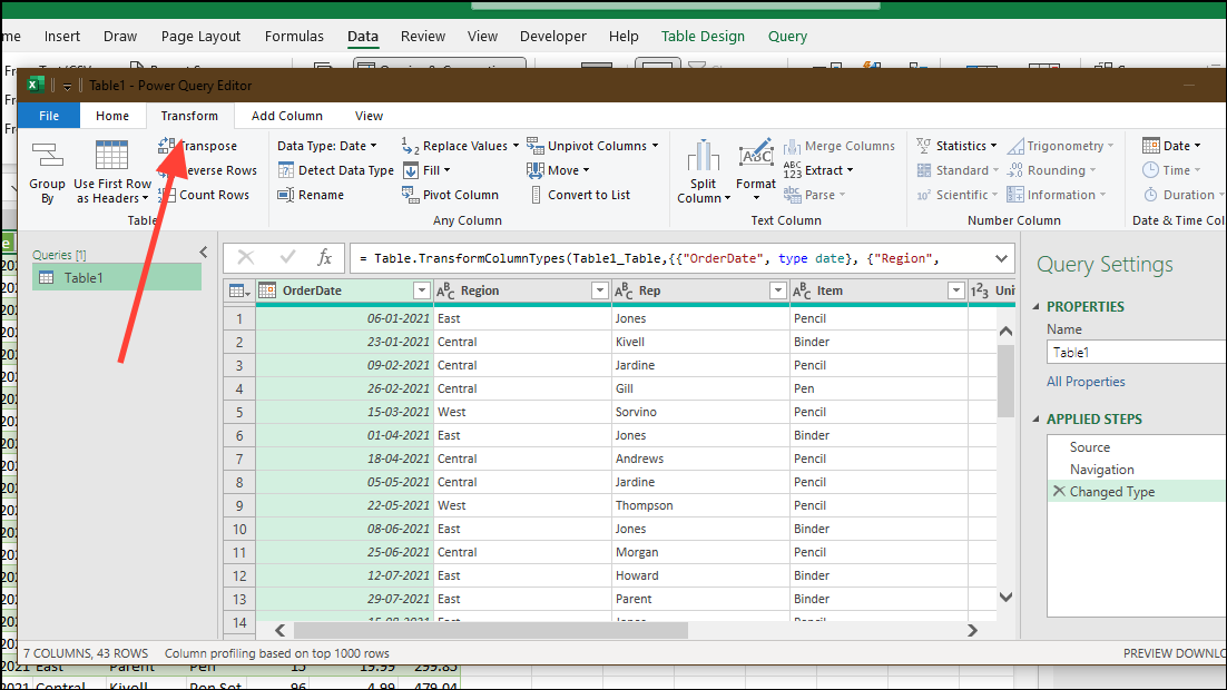
- After loading the data, go to the ‘Transform’ tab on the top, where you will find the ‘Transpose’ option.
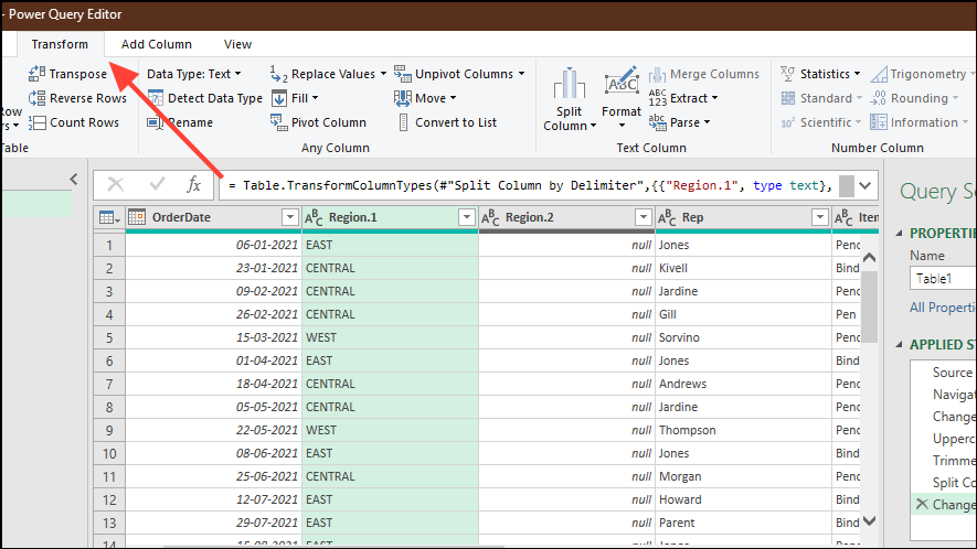
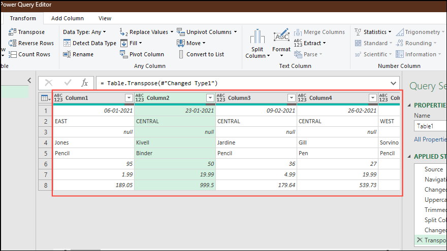
- Click the ‘Transpose’ option to convert the rows into columns.
Combining Queries
Power Query lets you easily combine multiple datasets using the ‘Merge’ and ‘Append’ options.
Using the Merge Option
The Merge operation lets you create a new query by combining existing queries.
- First, import the data into the Excel worksheet from a file, database, or other sources. In this case, you do not need to load the data into the Power Query Editor but will need to import multiple datasets.
- You will see another option, ‘Combine Queries’, beneath the options for importing data. Point your cursor to this option, and two options will be available – Append and Merge.
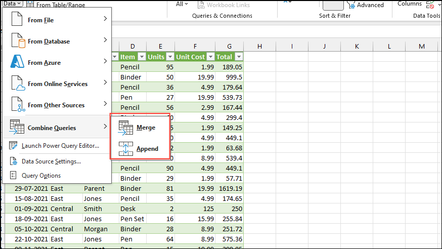
- Clicking the ‘Merge’ button will show you a new pop-up where you can select the datasets that have to be merged.
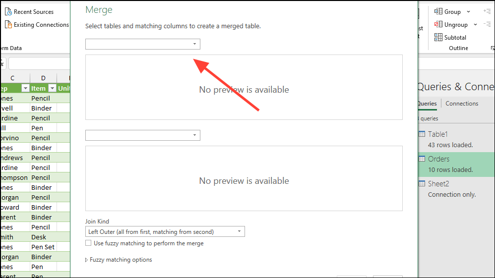
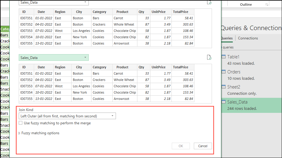
- Selecting the datasets will show you a preview. At the bottom left, you can select how you want to merge the datasets before clicking the ‘OK’ button.
Using the Append Option
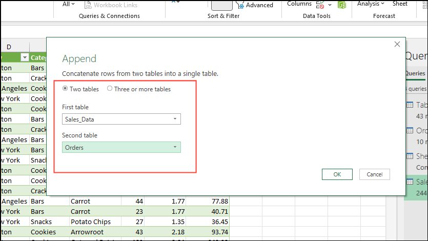
The ‘Append’ option allows you to create a new table by combining the rows of the previous queries.
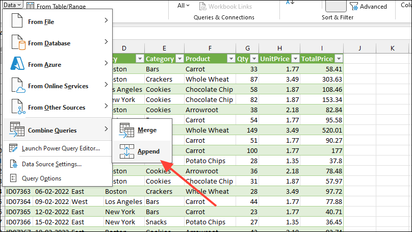
- Follow the same procedure as above to add the datasets to the Excel worksheet and then go to the ‘Append’ option in the ‘Combine Queries’ section.
- In the pop-up that comes up, select the tables for whom the data needs to be combined before clicking the ‘OK’ button. Users can combine data from two tables or from three or more tables.
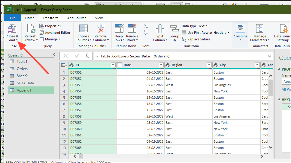
- The combined data will appear in the Power Query Editor window, from where you can import it into the worksheet using the ‘Close and Load’ button on the upper left side.
Loading Data to the Worksheet
When all your operations are complete in the Power Query Editor, you will need to load the data into your Excel worksheet.
- There are several ways to load the transformed data into your Excel worksheet, such as into a pivot chart, pivot table, table, or a connection for the query. Click the ‘Close and Load’ option in the upper left, and you will see two options – ‘Close and Load’ and ‘Close and Load To’.
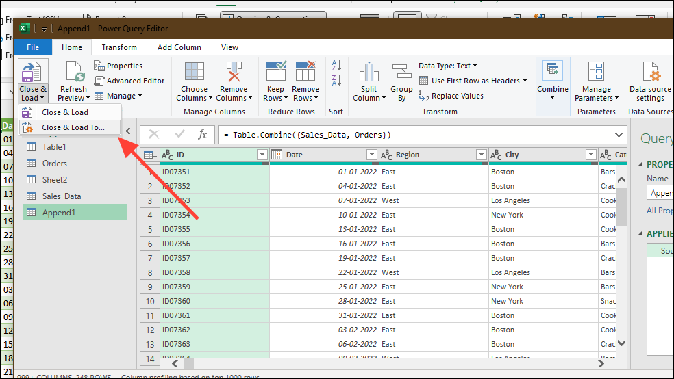
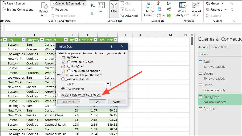
- Clicking the second option will show you the various options for loading the data into the worksheet.
- Excel allows you to choose the location, such as a cell in an existing worksheet or a new sheet that will be created automatically. There is also an option ‘Add This Data To The Data Model’.
Using Formulas and Functions
Power Query also allows the use of formulas and functions similar to Excel worksheets. This requires adding custom columns where you can add formulas and functions.
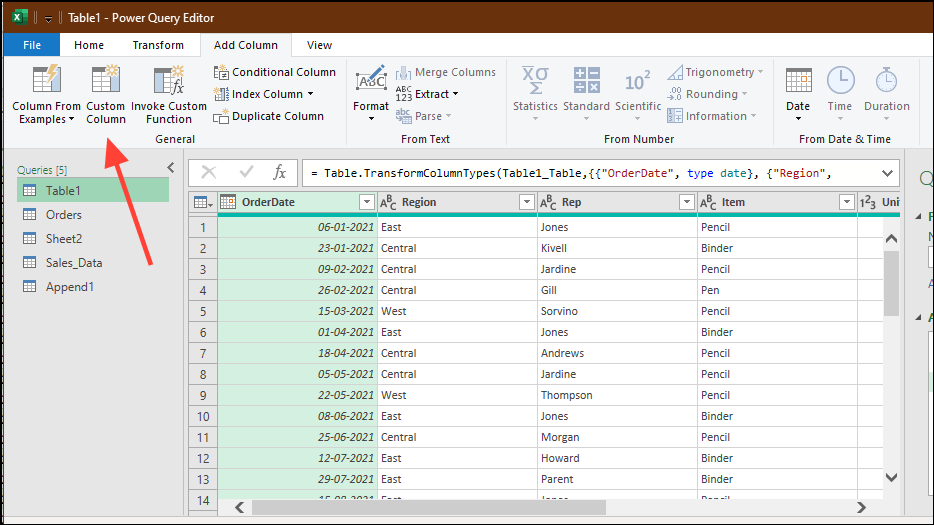
- Launch the Power Query Editor from the ‘Get Data’ tab and go to the ‘Add Column’ tab at the top.
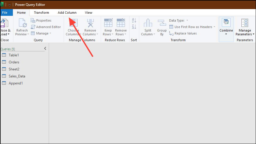
- On the left side, you will see your queries. Select one by clicking it, and the ‘Custom Column’ will become active. Create a new column by clicking the ‘Custom Column’ option.
- In the dialog box to create a Custom Column, provide a name for the column.
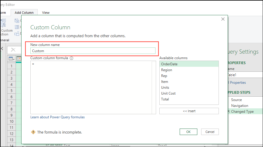
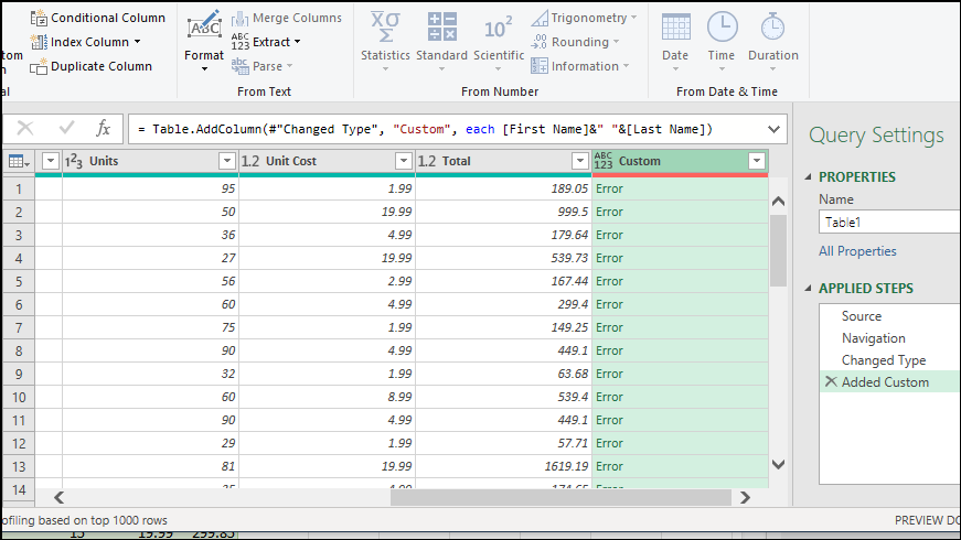
- In the ‘Custom Column Formula’ section, add a formula for creating the column. For instance, use a formula like
[First Name]&" "&[Last Name]. The Power Query Editor will verify whether there are any errors in the formula.
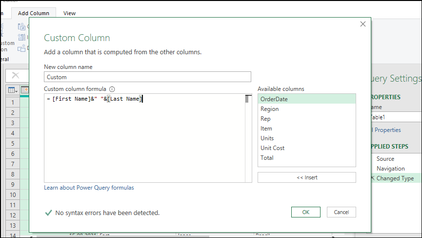
- If there are no errors, click the ‘OK’ button, and the editor will create a column.
- To use a function, repeat the steps till the ‘Custom Column’ pop-up appears. In the ‘Custom Column Formula’ section, add a function, such as
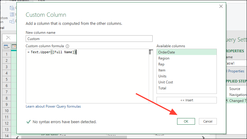
Text.Upper([Full Name]), which will create all names in the uppercase.
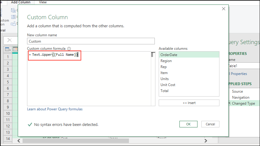
- To finish adding the column, click the ‘OK’ button to create a column with the names in uppercase.
That’s all you need to know to get started with Power Query. This tool makes it incredibly easy to transform data in Microsoft Excel as needed, so you can analyze and draw conclusions with minimal effort. It can be used to combine different datasets, change their formatting, and perform other actions. And you can even use Excel functions and formulas with the editor, which makes it even more useful.


