#SPILL! is a new kind of Excel error that mainly occurs when a formula that produces multiple calculation results trying to display its outputs in a spill range but that range already contains some other data.
The blocking data could be anything including, text value, merged cells, a plain space character, or even when there is not enough place to return the results. The solution is simple, either clear the range of any blocking data or select an empty array of cells that don’t contain any type of data in it.
Spill error usually happens when calculating dynamic array formulas, because the dynamic array formula is the one that outputs results into multiple cells or an array. Let’s look into more detail and understand what triggers this error in Excel and how to resolve it.
What causes a spill error?
Since, the launch of Dynamic arrays in 2018, Excel formulas can handle multiple values at a time and return results in more than one cell. Dynamic arrays are resizable arrays that allow formulas to return multiple results to a range of cells on the worksheet based on a formula entered in a single cell.
When a dynamic array formula returns multiple results, these results automatically spill into the neighboring cells. This behavior is called ‘Spill’ in Excel. And the range of cells where the results spill into is called the ‘Spill range’. The spill range will expand or contract automatically based on the source values.
If a formula is trying to fill a spill range with multiple results but is blocked by something on that range, then a #SPILL error occurs.
Excel now has 9 functions that use Dynamic Array functionality to solve problems, these includes:
- SEQUENCE
- FILTER
- TRANSPOSE
- SORT
- SORTBY
- RANDARRAY
- UNIQUE
- XLOOKUP
- XMATCH
Dynamic array formulas are only available in ‘Excel 365’ and it’s currently not supported by any of the offline Excel software (i.e. Microsoft Excel 2016, 2019).
Spill errors are not only caused by obstructing data, there are several reasons why you may get #Spill error. Let us explore the different situations where you might encounter the #SPILL! error and how to fix them.
Spill Range isn’t Blank
One of the primary causes for spill error is that the spill range is non-empty. For instance, if you are trying to display 10 results, but if there’s any data in any of the cells in the spill area, the formula returns a #SPILL! error.
Example 1:
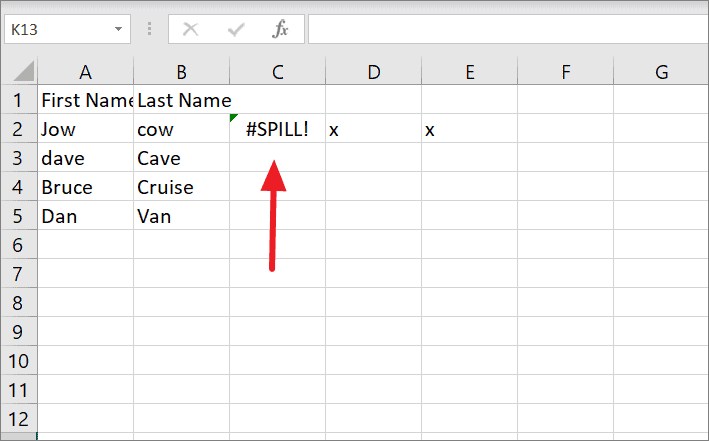
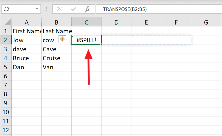
In the example below, we have entered the TRANSPOSE function in cell C2 to convert the vertical range of cells (B2:B5) into a horizontal range (C2:F2). Instead of switching the column to a row, Excel shows us the #SPILL! error.
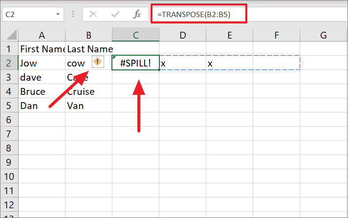
And when you click on the formula cell, you will see a dashed-blue border indicating the spill area/range (C2:F2) that is needed to display the results as shown below. Also, you will notice a yellow warning sign with an exclamation mark on it.
To understand the reason behind the error, click the warning icon next to the error and see the message in the first line highlighted in grey. As you can see, it says ‘Spill range isn’t blank’ here.
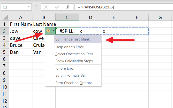
The problem here is that the cells in the spill range D2 and E2 have text characters (not empty), hence, the error.
Solution:
The solution is simple, either clear the data (either move or delete) located in the spill range or move the formula to another location where there is no obstruction.
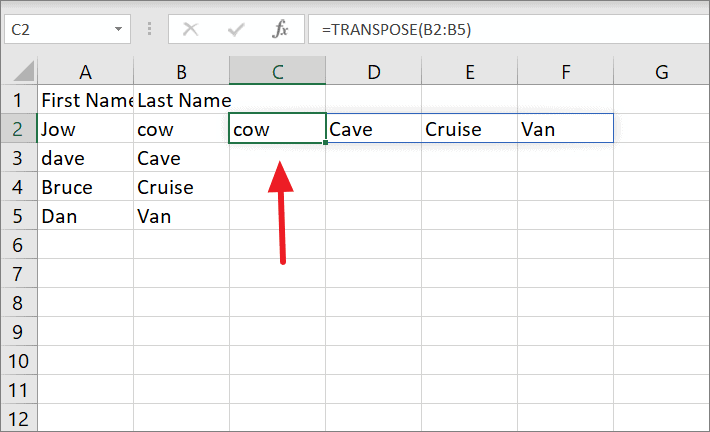
As soon as you delete or move the blockage, Excel will automatically populate the cells with the results of the formula. Here, when we clear the text in D2 and E2, the formula transposes the column to row as intended.
Example 2:
In the below example, although the spill range appears empty, the formula still shows the Spill! error. It is because the spill is not actually empty, it has an invisible space character in one of the cells.
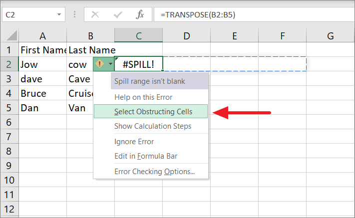
It’s hard to locate space characters or any other invisible character hiding in what appears to be empty cells. To find such cells with unwanted data, click the Error floatie (warning sign) and select ‘Select Obstructing Cells’ from the menu and it will take you to the cell that contains the obstructing data.
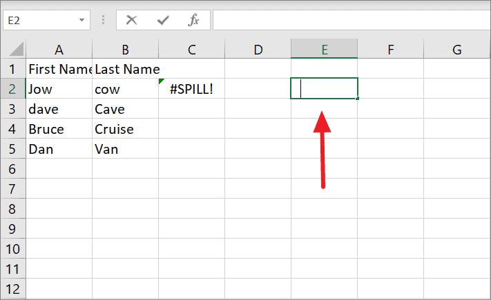
As you can see, in the below screenshot, cell E2 has two space characters. When you clear those data, you’ll get the proper output.
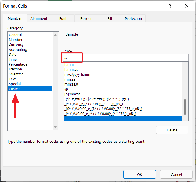
Sometimes, the invisible character could be a text formatted with the same font color as the cell’s fill color or a cell value custom formatted with the number code ;;;. When you custom format a cell value with ;;;, it will hide anything in that cell, regardless of font color or cell color.
Spill Range Contains Merged Cells
Sometimes, the #SPILL! error occurs when the spill range contains the merged cells. Dynamic array formula doesn’t work with merged cells. To fix this, all you have to do is unmerge cells in the spill range or move the formula to another range that has no merged cells.
In the below example, even though the spill range is empty (C2:CC8), the formula returns the Spill error. It’s because the cells C4 and C5 are merged.
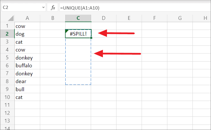
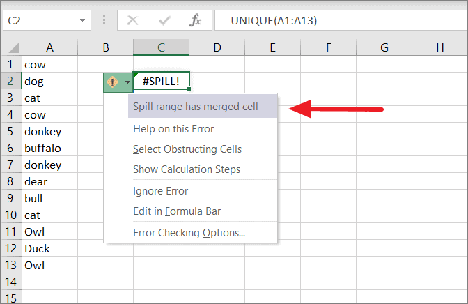
To make sure that merged cells are the reason you’re getting the error, click on the warning sign and verify the cause – ‘Spill range has merged cell’.
Solution:
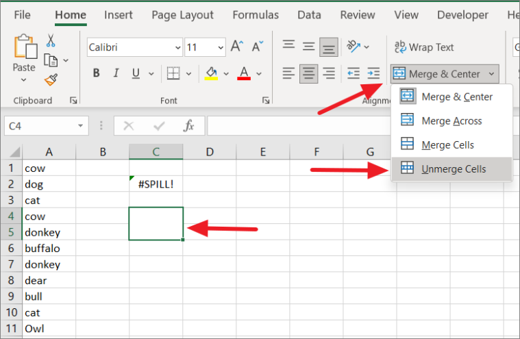
To unmerge the cells, select the merged cells, then on the ‘Home’ tab, click the ‘Merge & Center’ button and select ‘Unmerge Cells’.
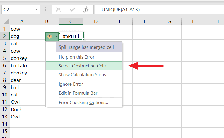
If you have a hard time locating the merged cells in your large spreadsheet, click on the ‘Select Obstructing Cells’ option from the warning sign menu to jump to the merged cells.
Spill Range in Table
Spilled array formulas are not supported in Excel tables. Dynamic array formula should only be entered in a single individual cell. If you enter a spilled array formula in a table or when the spill area falls into a table, you would get the Spill error. When this happens, try converting the table to a normal range or move the formula outside the table.
For example, when we enter the following spilled range formula in an Excel table, we would get a Spill error in every cell of the table, not just the formula cell. It’s because Excel automatically copies any formula entered in a table to every cell in the table’s column.
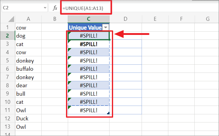
Also, you’ll get a spill error when a formula tries to spill results in a table. In the below screenshot, the spill area falls within the existing table, so we get a Spill error.
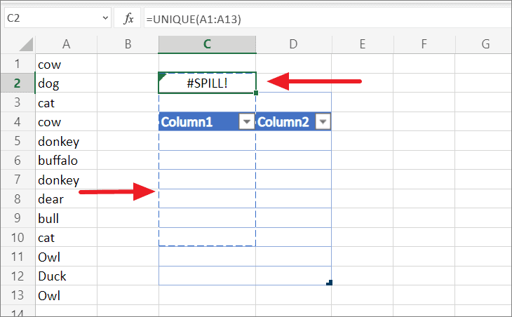
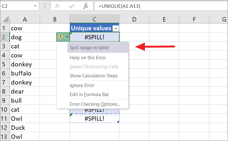
To confirm the cause behind this error, click the warning sign and see the error reason – ‘Spill range in table’
Solution:
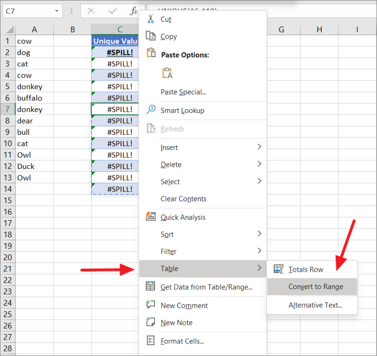
To fix the error, you’ll need to revert the Excel table back to the range. To do that, right-click anywhere within the table, click ‘Table’, and then select the ‘Convert to Range’ option. Alternatively, you can left-click anywhere within the table, then go to the ‘Table Design’ tab and select the ‘Convert to Range’ option.
Spill Range is Unknown
If Excel was unable to establish the size of the spilled array, it will trigger the Spill error. Sometimes, the formula enables a dynamic array to resize between each calculation passes. If the size of the dynamic array keeps changing during calculations passes and doesn’t balance out, it will cause the #SPILL! Error.
This type of Spill error is usually triggered when using volatile functions such as RAND, RANDARRAY, RANDBETWEEN, OFFSET, and INDIRECT functions.
For example, when we use the below formula in cell B3, we get the Spill error:
=SEQUENCE(RANDBETWEEN(1, 500))In the example, the RANDBETWEEN function returns a random integer between numbers 1 and 500, and its output is continuously changing. And the SEQUENCE function doesn’t know how many values to produce in a spill array. Hence, the #SPILL error.
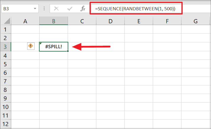
You can also confirm the cause of the error by clicking the Warning sign – ‘Spill range is unknown’.
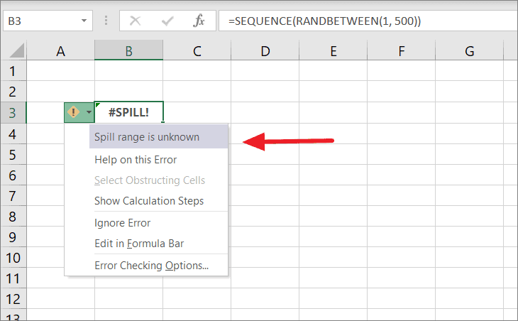
Solution:
To fix the error for this formula, your only choice is to use a different formula for your calculation.
Spill Range is Too Big
At times you may execute a formula that outputs a spilled range that is too big for the worksheet to handle, and it may extend beyond the edges of the worksheet. When that happens you may get #SPILL! error. To fix this issue, you can try referencing a specific range or one cell instead of entire columns or using the ‘@’ character to enable implicit intersection
In the example below, we’re trying to calculate 20% of the Sales numbers in column A and return the results in column B, but instead, we get a Spill error.
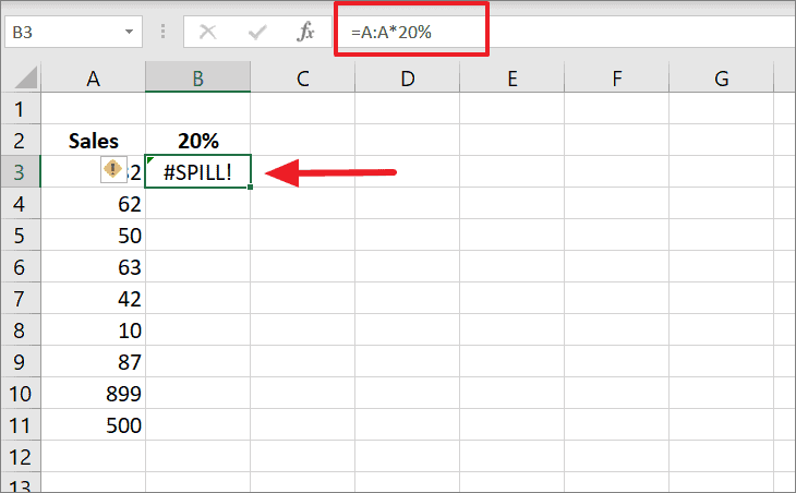
The formula in B3 calculates 20% of the value in A3, then 20% of the value in A4, and so on. It produces over a million results ( 1,048,576) and spills all of them in column B starting in cell B3, but it will reach the end of the worksheet. There isn’t enough space to show all the outputs, as a result, we get a #SPILL error.
As you can see the cause of this error is that the – ‘Spill range is too big’.
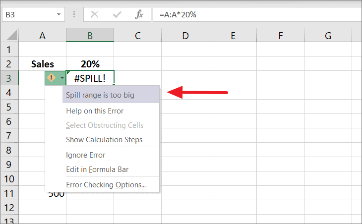
Solutions:
To solve this issue, try changing the entire column with a relevant range or a single-cell reference, or add the @ operator to perform implicit intersection.
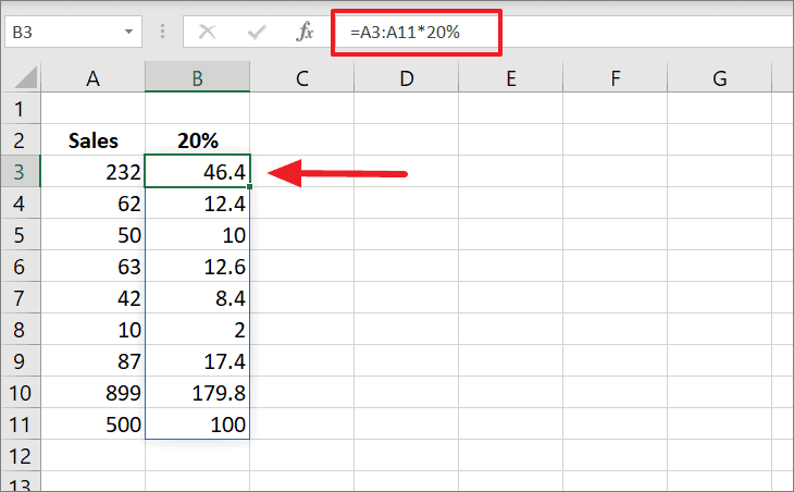
Fix 1: You can try referring ranges rather than entire columns. Here, we changing the entire range A:A with A3:A11 in the formula, and the formula will automatically populate the range with results.
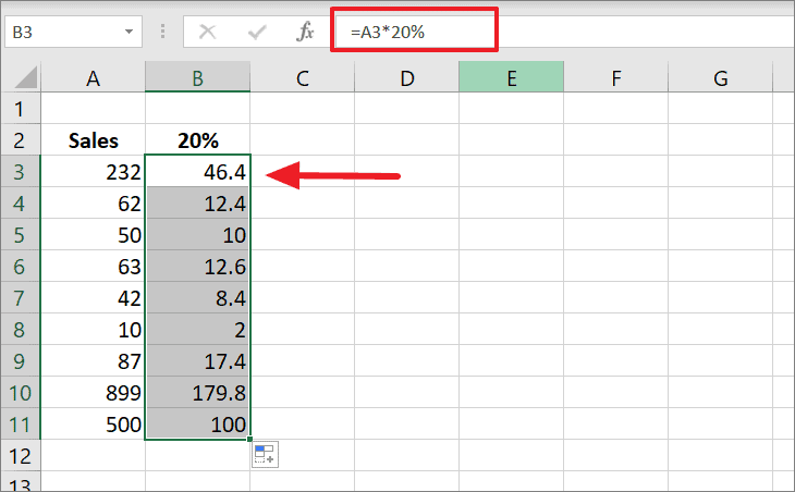
Fix 2: Replace the entire column with just the cell reference on the same row (A3), and then copy the formula down the range using the fill handle.
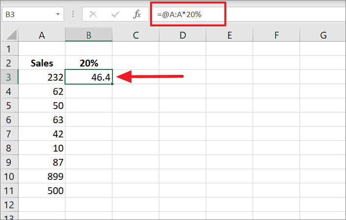
Fix 3: You can also try adding the @ operator before the reference to perform implicit intersection. This will display the output in the formula cell only.
Then, copy the formula from cell B3 to the rest of the range.
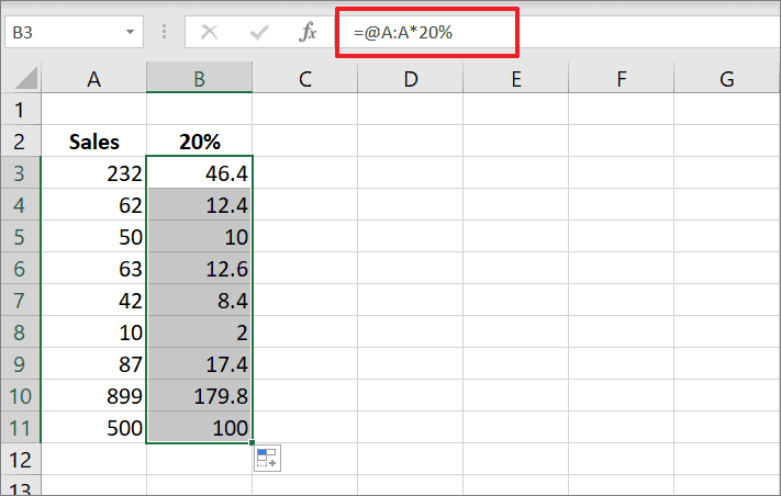
Note: When you are editing a spilled formula, you can only edit the first cell in the spill area/range. You can see the formula in other cells of the spill range, but they will be greyed out and cannot be updated.
Out of memory
If you execute a spilled array formula that causes Excel to run out of memory, it may trigger the #SPILL error. Under those circumstances, try referencing a smaller array or range.
Unrecognized / Fallback
You can also get a Spill error even when Excel does not recognize or cannot reconcile the cause of the error. In such cases, double-check your formula and make sure all parameters of the functions are correct.
Now, you know all the causes and solutions for #SPILL! errors in Excel 365.

