
In statistics, Standard Deviation is used to find how far each value in a data set varies from the mean or average value. This helps us understand how closely each number is clustered around the mean.
There are several types of professionals who use standard deviation as a fundamental risk measure, such as Insurance analysts, portfolio managers, Statisticians, Market researchers, Real estate agents, stock investors, etc.
However, calculating Standard Deviation in Excel can be a daunting process for those who are new to Excel or aren’t familiar with it. That is why, in this article, we are going to explain what Standard Deviation is and how to calculate it in Excel.
What is Standard Deviation?
The mean value indicates the average value in the data set. And the Standard Deviation represents the difference between the values of the data set and their average value. In other words, standard deviation tells you whether your data is close to the mean or varies a lot.
For example, if a teacher were to tell you that the average score of her students is 60 (mean). And if you have the list of her students’ scores, you can use standard deviation to find out how accurate she is.
There are two types of Standard deviations: population standard deviation and sample standard deviation. The sample standard deviation (SSD) is calculated from the random samples of the population or data while population standard deviation (PSD) is calculated from the entire population data.
The higher the standard deviation, the more spread out the data is from the mean, and the lower the standard deviation, the closer the values are to the average/mean. If the standard deviation is 0, all the data points in the data set are equal. Also, a higher standard deviation means the mean is less accurate, and a lower standard deviation indicates the mean is more reliable.
There are two different ways for calculating Standard Deviation in Excel using formulas or built-in functions.
Population vs. Sample
Sample calculations are common because sometimes it’s not possible to calculate the entire data set. Before you start calculating standard deviation, you must know what kind of data you have – entire data or sample of the data. Because you have to use different formulas and functions for sample and population data.
- Population data refers to the entire data set. It means the data is available for all the members of a group. The population standard deviation calculates the distance of each value in a data set from the population mean. An example of population data is a census.
- Sample data on other hand is the subset of the population. It is a subset that represents the entire population. The sample is a smaller group of data that is derived from the population. Sample data is used when the entire population is not available or it is enough for statistics. A good example of a sample is a survey.
Calculate Standard Deviations using Manual Calculations
Manually calculating standard deviations is a bit of a lengthy process, but can be easily done using formulas. First, you need to calculate the variance of data and then find the square root of the variance.
Population Standard Deviation
The formula for calculating the population standard deviation is given below:
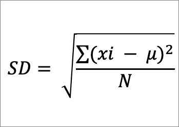
Where
- μ is the arithmetic mean
- Xi is individual values in the set of data
- N is the total number of X values (population) in the data set
Sample Standard Deviation
The formula for calculating the sample standard deviation is given below:
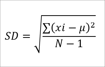
Where
- μ is the arithmetic mean
- Xi is individual values in the sample data set
- N is the total number of X values (sample) in the data set
When calculating sample standard deviation, only the sample of the data set is considered from an entire data set. Hence, Bessel’s correction (N-1) is used instead of N to give a better estimation of the standard deviation.
To calculate the standard deviation for the below data set, follow these steps:
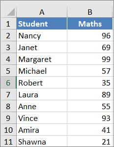
1. Calculate the Mean (Average)
First, you need to calculate the mean/average (μ) of all values in the data set. To do that, you add up all the values and then divide the sum by the count of the values in the data set. You can find the average using the manual arithmetic expression:
96+69+99+57+35+89+55+93+41+21/10=65.5You can also use the AVERAGE function in Excel to calculate the mean:
=AVERAGE(B2:B11)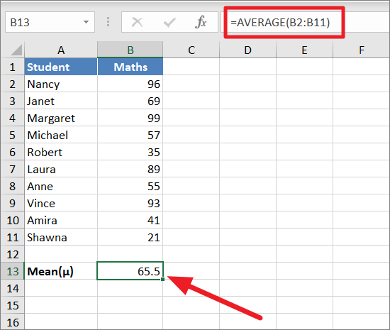
Here, B2:B11 in the formula represents the cells (denoted as the column number followed by the row number) that hold the data for which we intend to calculate the mean. Replace these values with the cells in your sheet while using the formula.
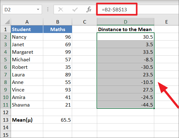
2. For Each Number, Calculate the Distance to the Mean:
After that, you need to find the deviation or distance to the mean by subtracting the Mean from each value in the data set. To do that, enter the below formula:
=B2-$B$13or
=(B2-AVERAGE(B2:B11))$B$13 is the mean of the data. The above formula is entered in cell D2 and then applied to the whole column by dragging it downwards to find the deviation for the whole column (D2:D13). Place your cursor at the bottom-right corner of the cell, here D2. A ‘+’ symbol will appear; drag it downward.
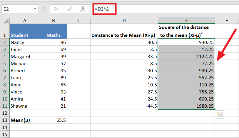
3. Square the difference
Now, square the difference for each value by using the below formula:
=D2^2Then apply the formula to the whole column by dragging it downward. Squaring the difference will also turn the negative values into positive values.
4. Sum the Squared Differences
Next, sum all the squares of the deviation about the mean (Xi-μ)2. Here’s the formula for adding up the squared differences:
=SUM(E2:E11)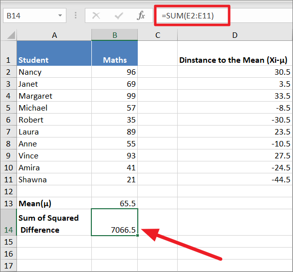
If you have large data set, you can calculate the count of values by:
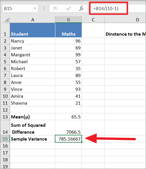
=B14/105. Calculate the Variance
To calculate the variance, you need to divide the squared difference by the number of values.
So far, the steps for calculating sample and population standard deviation were the same. In this step, the formulas are going to change a little for both standard deviations, as explained before.
For sample variance, you need to divide the sum of squared differences by the number of values minus 1:
=B14/(10-1)or
=SUM(E2:E11)/(COUNT(B2:B11)-1)You can use either of the formulas to calculate sample variance.
For population variance, you need to divide the sum of squared differences by just the number of values:
=B14/10or
=SUM(E2:E11)/(COUNT(B2:B11)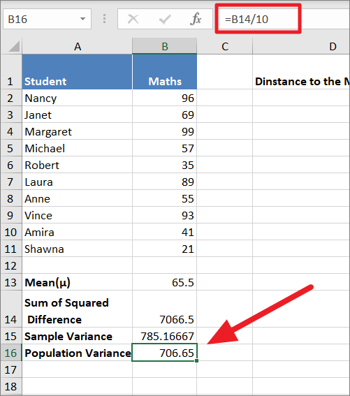
6. Get the Square Root of the Variance
Finally, you need to take a square root of the above variance to get the Standard Deviation.
Sample Standard deviation:
To get the sample standard deviation, take the square root of the sample variance:
=SQRT(B15)or
=SQRT(SUM(E2:E11)/(COUNT(B2:B11)-1))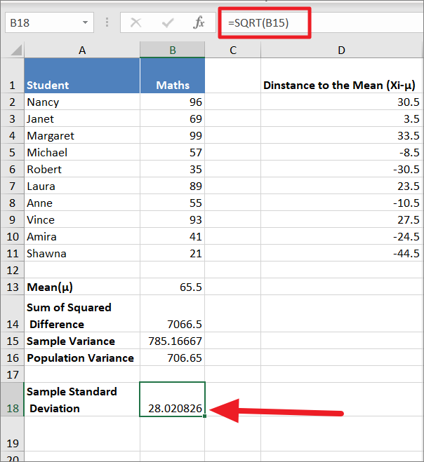
Population Standard Deviation:
To get population standard deviation, calculate the square root of the population variance:
=SQRT(B16)or
=SQRT(SUM(E2:E11)/COUNT(B2:B11))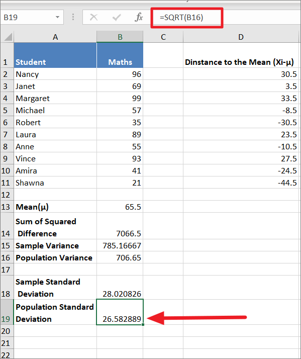
Calculate the Standard Error in Excel
The standard error of the mean or simply the standard error is another measure of variability, very similar to standard deviation, yet different. It is a measure of how far each population means is likely to be from a sample mean.
The difference between standard error and the standard deviation is that standard error uses statistics (sample data) while standard deviation uses parameters (population data). The Standard Deviation usually measures the variability within a single sample while Standard Error measures variability across multiple samples of a population. Here’s how you can calculate Standard Error (SE):
The general formula for standard error is the standard deviation divided by the square root of the number of values in the data set.
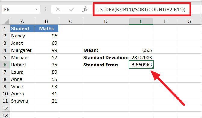
= Sample Standard Deviation / Square root of number of values (n)To calculate Standard Error (SE), enter the below formula:
=STDEV(B2:B11)/SQRT(COUNT(B2:B11))Here, STDEV(B2:B11) finds the standard deviation of the sample (B2:B11), and the SD is divided by the square root of the number of values (n) in B2:B11. Instead of COUNT(B2:B11), you can also directly type in the number of values in the data set (10).
Calculate the Standard Deviation using Excel Built-in Functions
Microsoft Excel includes six different functions for calculating standard deviation. These functions make it extremely easy to calculate the Standard Deviation in Excel, cutting down on the time you need to spend on the calculations. The only catch is that you need to know which function to use when. The function you need to use depends upon the data you have – sample or population.
When you type =STDEV in a blank Excel cell, it will show you the following six versions of the standard deviation functions:
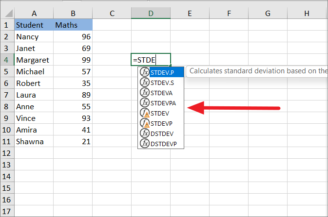
- STDEV: It is used for calculating the standard deviation for sample data. This function is the oldest Excel function (before Excel 2007) for finding standard deviation. This still exists in the latest Excel versions for compatibility purposes.
- STDEVP: This is another older version of the standard deviation that exists for compatibility with Excel 2007 and earlier. It calculates standard deviation based on the population data.
- STDEV.S: This is a newer version of the STEDV function (available since Excel 2010). It is used for calculating the standard deviation for sample data.
- STDEV.P: This is a newer version of the STEDVP function in Excel (available since Excel 2010). It is used for calculating the standard deviation for entire population data.
- STDEVA: This formula calculates the sample standard deviation of a dataset by including text and logical values. It is very similar to STDEV.S. All FALSE values and Text values are taken as ‘0’ and TRUE is taken as ‘1’.
- STDEVPA: This formula calculates the population standard deviation by including text and logical values. It is similar to STDEV.P. All FALSE values and Text values are taken as ‘0’ and TRUE is taken as ‘1’.
STDEV, STDEVP, STDEV.S, STDEV.P ignores the text and logical (TRUE or FALSE) values in the dataset. In most cases, you will only need STDEV.P or STDEV.S to perform standard deviation calculations.
To give you a better understanding, here’s a summary of the six functions:
| Function name | Standard Deviation | Handling of Logical & Text values | Excel version |
|---|---|---|---|
| STDEV.S | Sample standard deviation | Ignored | 2010 – 2021 |
| STDEV.P | Population standard deviation | Ignored | 2010 – 2021 |
| STDEV | Sample standard deviation | Ignored | 2003 – 2021 (Available for compatibility with 2007 and earlier) |
| STDEVP | Population standard deviation | Ignored | 2003 – 2021 (Available for compatibility with 2007 and earlier) |
| STDEVA | Sample standard deviation | Evaluated (TRUE=1, FALSE=0, Text = 0) | 2003 – 2021 |
| STDEVPA | Population standard deviation | Evaluated (TRUE=1, FALSE=0, Text = 0) | 2003 – 2021 |
Excel STDEV.P Function for Population Standard Deviation
If your data set represents the entire population, you can use the STDEV.P function to calculate the population standard deviation.
The syntax for the STDEV.P function is:
=STDEV.P(number1,[number2],…)Where
- number1 is the first number argument that corresponds to the first data point of the population data.
- [number2],.. is the second number argument that corresponds to the second data point of the population data and so on.
The function must contain two or more values in the arguments and the function can take up to 255 numeric arguments. You can input numbers, arrays, and cell references as arguments.
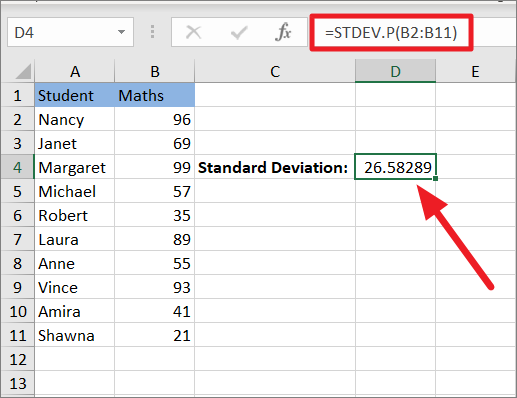
Example:
=STDEV.P(B2:B11)Here, B2:B11 is the range of cells that contains the population data. The above formula will return the standard deviation for the given population. As you can see, we get exactly the same result 26.58289 (population standard deviation) as the above manual method. This function automatically performs all the step-by-step calculations from the above manual method in the background and gives you the result.
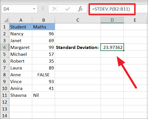
In case your data contains any boolean values (TRUE or FALSE) or text values, this function ignores those values and calculates the standard deviation with the remaining values.
As you can see below, the same above formula produced a different result because it ignored the values in the cells B8 and B11.
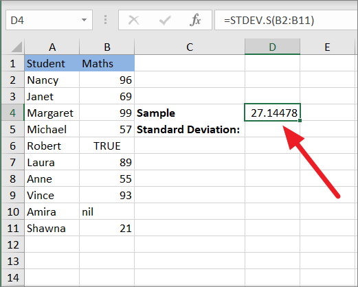
Excel STDEV.S Function for Sample Standard Deviation
If your data set represents the sample population, you can use the STDEV.S function to calculate the sample standard deviation. For example, you have conducted a test for a large number of students but you only have a test score of 10 students, so you can use STDEV.S to find the sample standard deviation and apply it to the entire population.
The syntax for the STDEV.S function is:
=STDEV.S(number1,[number2],…)Where
- number1 is the first number argument corresponding to the first data point of the sample data.
- [number2],… is the second number argument that corresponds to the second data point of the sample data and so on.
You can input numbers, arrays, and cell references as arguments.
Example:
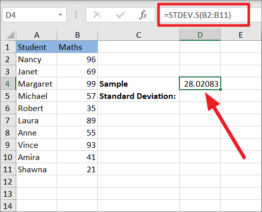
=STDEV.S(B2:B11)The above formula sums up all the squares of the deviation about the mean and divides it by the count minus 1 (n-1) in the background and returns the below result.
STDEV.S function also ignores the text and logical values if there are any in the data set as shown below.
Excel STDEVA Function for Sample Standard Deviation
The STDEVA is another function used to calculate the standard deviation for a sample, but it differs from the STDEV.S only in the way it handles logical and text values.
In all the above functions, logical values and text values are ignored, but the STDEVA function converts those values into 1s and 0s.
- The logical values TRUE are counted as ‘1’ and FALSE are counted as ‘0’. The values can be contained within cells, arrays, or entered directly into the function as arguments.
- All text strings including empty strings (“”), text representations of numbers, and any other text are evaluated as ‘0’.
To evaluate the standard deviation for a sample, including logical values and text, use this formula:
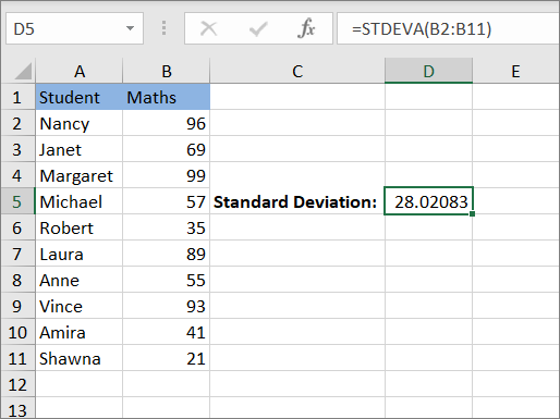
=STDEVA(B2:B11)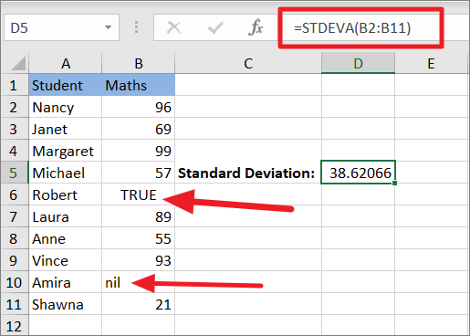
If there are no logical or text values in the data set, it will return the usual standard deviation.
Excel STDEVPA Function for Population Standard Deviation
Excel also has a function called STDEVPA for calculating standard deviation for a population by including text and logical values. This function is similar to the STDEVA in handling text and boolean values.
- The logical values TRUE are counted as ‘1’ and FALSE are counted as ‘0’.
- All text strings including empty strings (“”), text representations of numbers, and any other text are evaluated as ‘0’.
To evaluate standard deviation for a population, including logical values and text, use the below formula:
=STDEVPA(B2:B11)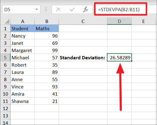
Excel STDEV Function
Excel’s STDEV Function is very similar to the STDEV.S function, it can calculate the standard deviation for sample data. If you are working in Excel 2007 or earlier version, you need to use the STDEV function to calculate the standard deviation.
Syntax for STDEV function:
=STDEV(number1, [number 2],...)Example:
=STDEV(B2:B11)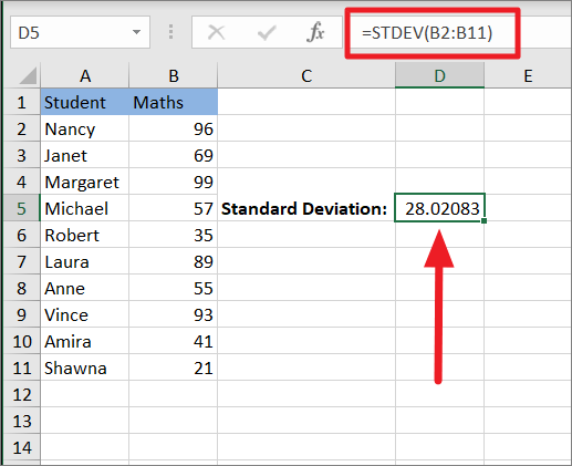
STDEV function exists in the newer versions of Excel for compatibility purposes which means it will be removed in the future. So, Microsoft is recommending that users use STDEV.S instead of STDEV.
Excel STDEVP Function
Excel’s STDEVP Function works exactly the same way as the STDEV.P function. If you are working in Excel 2007 or earlier version, you have to use the STDEVP function to calculate the standard deviation for population data.
The Syntax for STDEVP function:
=STDEVP(number1, [number 2],...)Example:
=STDEVP(B2:B11)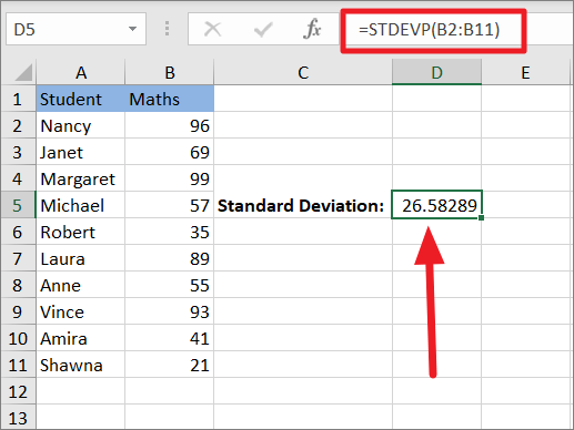
STDEVP may also be removed from the future Excel version.
Calculate Standard Deviation in Excel Using Insert Function
If all these functions are hard to remember, you can use the Insert Function option to quickly calculate the standard deviation. Also, you can avoid errors while writing the formula by using the Insert function feature to automatically insert the desired formula in your chosen result cell. Here’s how you can do that:
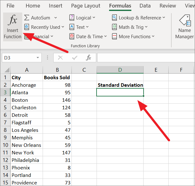
First, select the cell where you want the output. Then, go to the ‘Formulas’ tab and select the ‘Insert Function’ button in the ribbon.
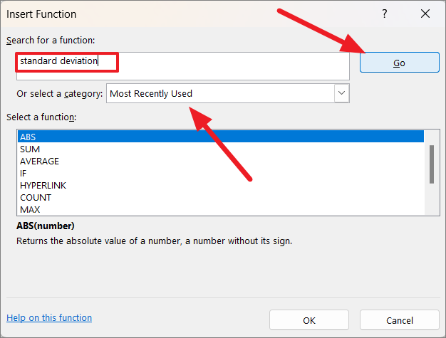
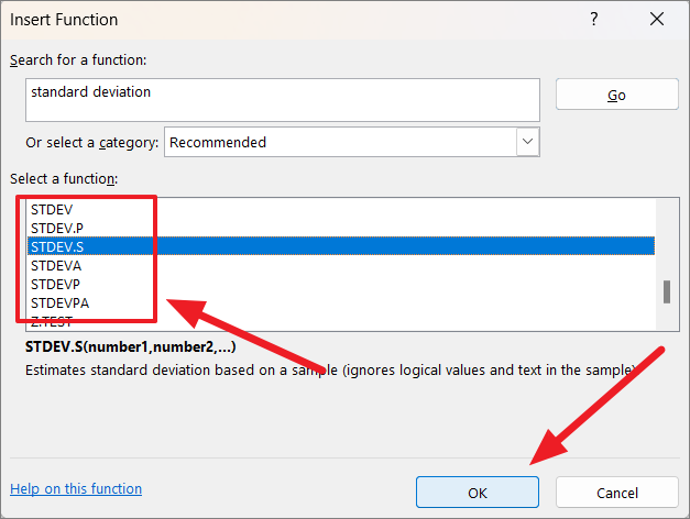
This will open the Insert Function dialog box. There, search for ‘Standard Deviation’ in the ‘Search for a function’ field or choose the ‘Statistical’ category from the ‘Or select a category’ drop-down, and click ‘Go’.
Then, scroll down the list of functions within the ‘Select a function’ window, choose a standard deviation function (STDEV.P, STDEV.S, STDEVA, or STDEPA), and click ‘OK’.
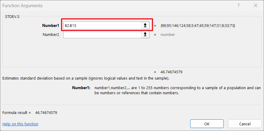
This will open up Function Arguments dialog windows with two fields Number 1 and Number 2. In the Number 1 field, enter the range for which you want to calculate the standard deviation. Or, click the upward-facing arrow in the text field and highlight the range from the worksheet. Each number argument can only take up to 255 cell counts. If the number of cells exceeds 255, you can use Number 2, Number 3, etc.
Then, click ‘OK’.
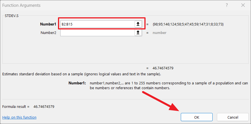
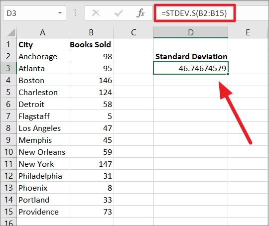
Once you click OK, it will calculate the standard deviation using the selected function and show you the result in the cell you originally selected.
Get Standard Deviation using Data Analysis Tool in Excel
You can also get standard deviation as part of the Descriptive Statistics summary of your data using the data analysis tool. Excel’s Data Analysis tool can automatically generate various key statistical values, including mean, median, Variance, standard deviation, standard error, etc.
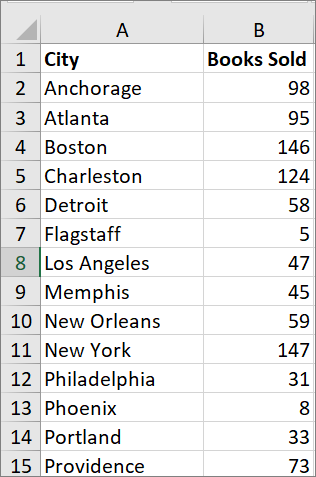
For the below data set, we want to calculate descriptive statistics. Here’s how you can do that:
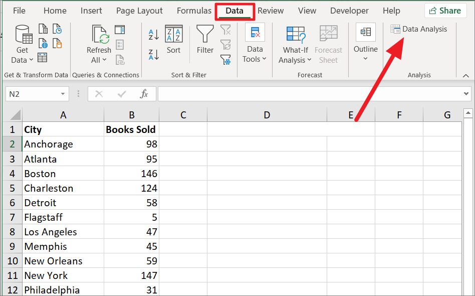
To get Descriptive Statistics, go to the ‘Data’ tab and click the ‘Data Analysis’ tool from the Analysis section.
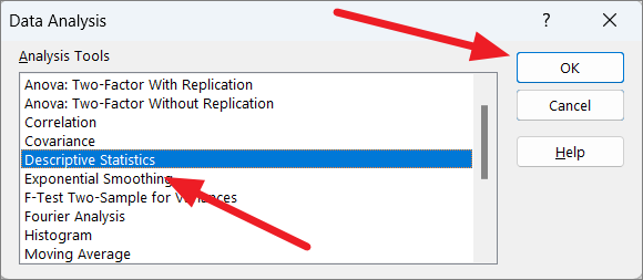
In the Data Analysis dialog window, select ‘Descriptive Statistics’ under Analysis Tools and click ‘OK’.
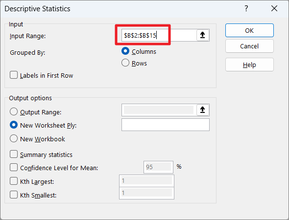
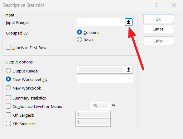
This will open the Descriptive Statistics dialog box in which you need to configure the Input and Output options.
Input Options
First, enter the range of variables/values you want to analyze in the ‘Input Range’ field.
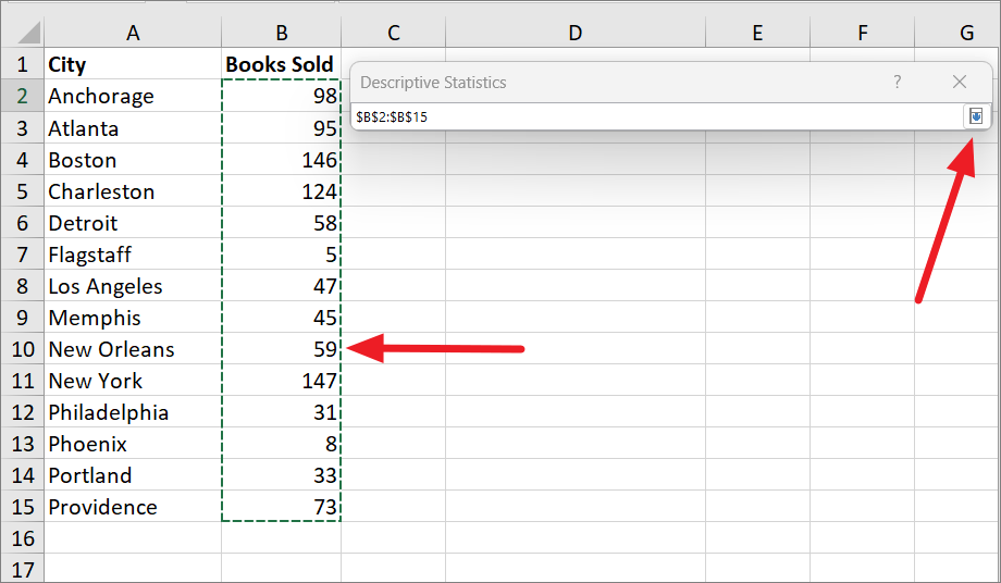
You can manually enter the range in the field or click the upward-facing arrow button at the end of the field to choose a range.
After that, select the range from the sheet and click the downward arrow button to confirm the range.
Next, choose how you want to organize your variables (rows or columns). Here, we are selecting ‘Columns’ because our input range is in columns.
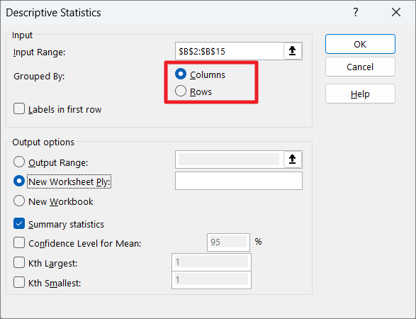
If you selected or entered the range (in the Input Range) with headers, you should tick the ‘Labels in first row’ option.
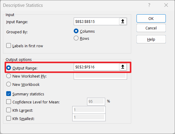
Output Options:
In the ‘Output Range’ field, enter the range where you want to display the statistical result. If you want to display the result in the current worksheet or another worksheet in the current workbook, click the ‘Output Range’ radio button and specify the range in the field next to it.
If you want to show the results in a new spreadsheet, simply select the ‘New Worksheet Ply’ radio button. Or, if you want to display the results in a new workbook, select the ‘New Workbook’ option.
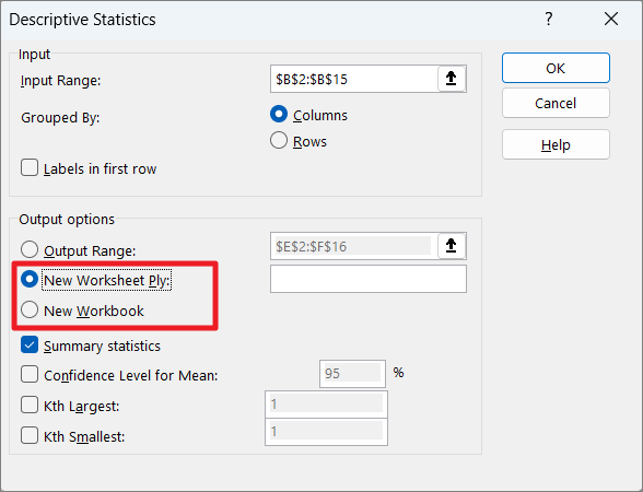
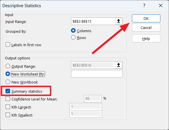
Finally, check the ‘Summary statistics’ option and click ‘OK’.
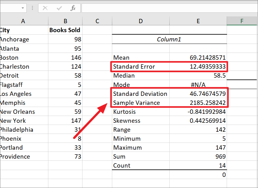
And you will get all the necessary statistics you want including Standard Error, Standard Deviation, Sample Variance, etc.
How to Calculate Standard Deviation with an IF Criteria
Besides the above-mentioned six Standard Deviation functions, Excel also has two more functions called DSTDEV and DSTDEVP for calculating standard deviation with an IF condition.
- DSTDEV function is used for calculating the standard deviation of data that is extracted from the sample data set matching the given criteria.
- DSTDEVP function is used for calculating the standard deviation of data that is extracted from the population data set matching the given criteria.
DSTDEV Function for Sample Standard Deviation
The syntax for the DSTDEV function:
=DSTDEV(database, field, criteria)- Database – The range of cells (table) where the data entries with values you want to calculate standard deviation are from. The range must include headers in the first row.
- Field: This specifies the field or column where the numbers you want to calculate the standard deviation are located. You need to specify the field name (i.e. column label or header) enclosed in double quotes or field number (i.e. column number) within the table.
- Criteria: The range of cells that contains where your criteria are. The criteria range must contain at least one column label matching your database headers and one cell below the column label that specifies the condition from the column. It can include multiple rows to specify multiple conditions.
Example:
Suppose you have the below dataset where you need to calculate standard deviation based on conditions:
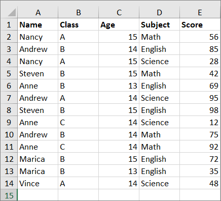
Example:
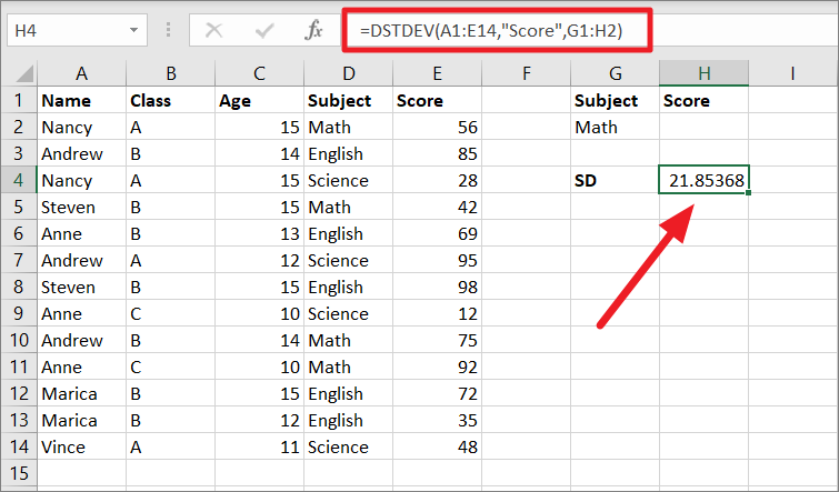
For example, to find the sample standard deviation of scores obtained in math subject by all students, enter either of the below formulas:
=DSTDEV(A1:E14,"Score",G1:H2)or
=DSTDEV(A1:E14,5,G1:H2)The above formula finds all the scores corresponding to Math and calculates the standard deviation for those scores. You need to create a separate criteria range (G1:H2) as shown below and enter the formula in an empty cell.
DSTDEVP Function for Population Standard Deviation
The syntax for the DSTDEVP function:
=DSTDEVP(database, field, criteria)Where
- Database – The range of cells (table) where the data entries with values you want to calculate standard deviation are from.
- Field: This specifies the field or column where the values you want to calculate the standard deviation are located.
- Criteria: The range of cells that contains where your criteria are.
Example 1:
For example, to find the population standard deviation of scores obtained in math subject by all students, enter the below formulas:
=DSTDEVP(A1:E14,"Score",G1:H2)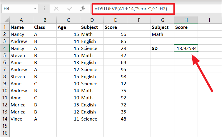
Example 2:
To find the population standard deviation of scores obtained in the math subject by students who are 14 and older, enter the below formula:
=DSTDEVP(A1:E14,"Score",G1:I2)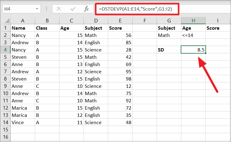
Wildcards
You can also use the following wildcards in the text related criteria to calculate standard deviation:
*– Matches any character with any amount?– Matches any single character~– Finds * or ? character in the search.
Multiple-row Criteria
You can include more than one row or column in the criteria range to calculate standard deviation using OR or AND logic. If you add more than one row in the criteria range, the functions will use OR logic (TRUE if at least one of the conditions is TRUE) to calculate the standard deviation. Whereas if you add more than one column in the criteria range, the functions will use the AND logic (TRUE if all of the conditions are TRUE) to evaluate.
=DSTDEV(A1:E14,"Score",G1:G3)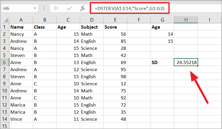
Calculate Weighted Standard Deviation in Excel
Normally, when we calculate a standard deviation for a data set, all the values in the data set carry equal weights or importance. However, in some cases, each value has a different weight in the data set and some values have higher weights than others because some values are more important than others.
In such cases, you cannot use the above built-in functions to calculate the standard deviation. So, you need to use other SUM, SUMPRODUCT, and SQRT functions to calculate the weighted standard deviation manually. Let us see how to calculate weighted standard deviation in Excel.
Suppose you have a dataset where the first column contains data values and the second column contains weights of each of those values:
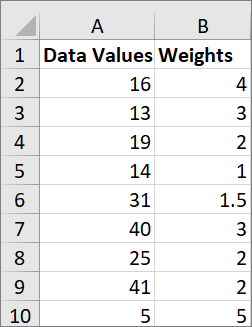
First, you need to calculate the weighted mean or average for the given data. You can do that with the following formula:
=SUMPRODUCT(value_range, weight_range)/SUM(weight_range)Where,
- value_range – Range or array of numbers.
- weight_range – Range cells with weights
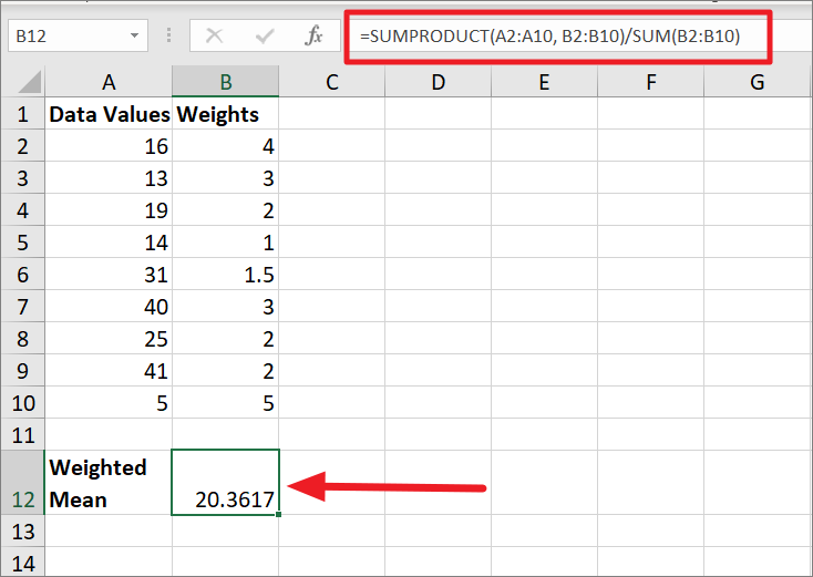
Example:
=SUMPRODUCT(A2:A10, B2:B10)/SUM(B2:B10)In the above formula, the SUMPRODUCT function multiplies each of the values (column A) with its weight (column B) and sums up the results. Then, the SUMPRODUCT result is divided by the sum of the data weights to produce the weighted mean.
Once you have the weighted mean, you can calculate the weighted standard deviation.
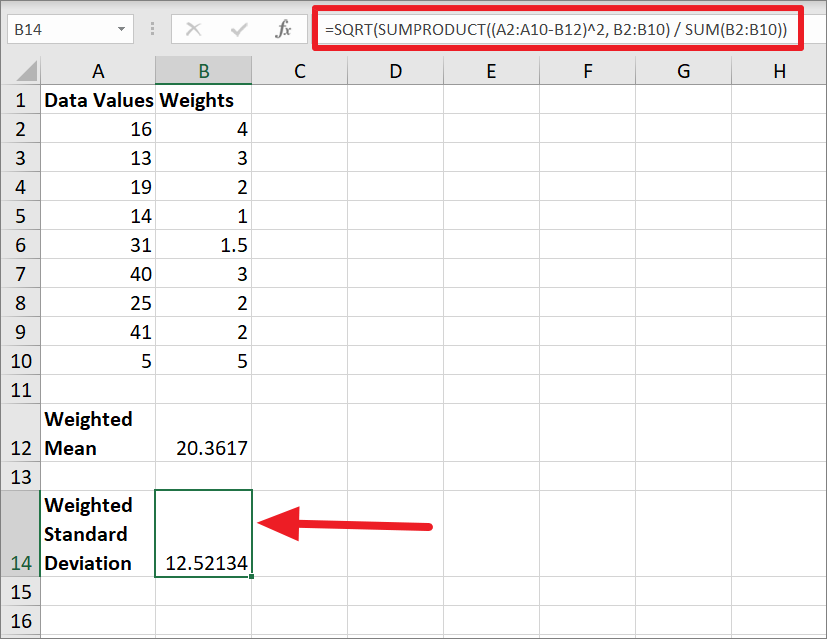
To calculate the standard deviation for population data, enter the below formula:
=SQRT(SUMPRODUCT((value_range - weighted_mean)^2, weight_range)/SUM( weight_range))Example:
=SQRT(SUMPRODUCT((A2:A10-B12)^2, B2:B10)/SUM(B2:B10))In the above formula, the calculated weighted mean is subtracted from each data value (column A) and each result is squared. After that, each square result is multiplied by data weight (column B) using the SUMPRODUCT function.
Then, the SUMPRODUCT result is divided by the SUM of the weights. After that, the square root of the result is calculated using the SQRT function to find the standard deviation value.
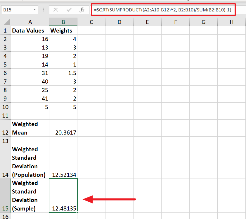
To calculate the standard deviation for sample data, enter the below formula:
=SQRT(SUMPRODUCT((value_range - weighted_mean)^2, weight_range)/SUM( weight_range)-1)Example:
=SQRT(SUMPRODUCT((A2:A10-B12)^2, B2:B10)/SUM(B2:B10)-1)The only difference in this formula from the above formula is that we added ‘-1’ to the sum of weight for the population data.
Add Standard Deviation Bars In Excel
You can also add standard deviation bars to visualize the margin of your standard deviation using Excel error bars. Excel errors are part of the chart elements that let you represent data variability and measurement. To add standard deviation bars to your chart, follow these steps:
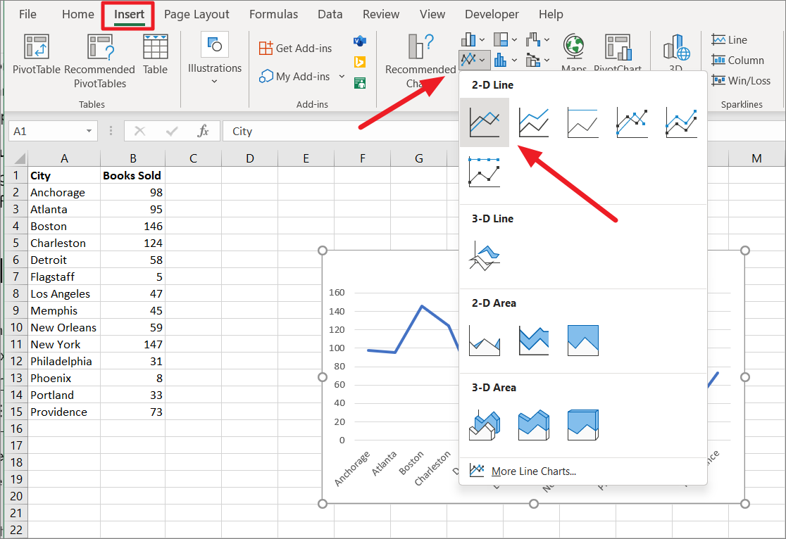
First, create a chart or graph for your data set. To do that, select the range of cells, go to the ‘Insert’ tab and choose a graph option from the Charts group.
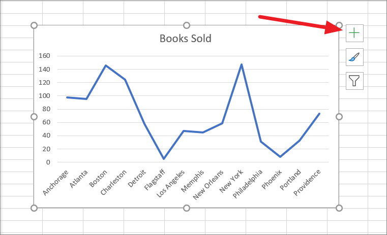
Once the chart is inserted, select the graph by clicking anywhere on the graph, then click the ‘Chart Elements’ (+) button.
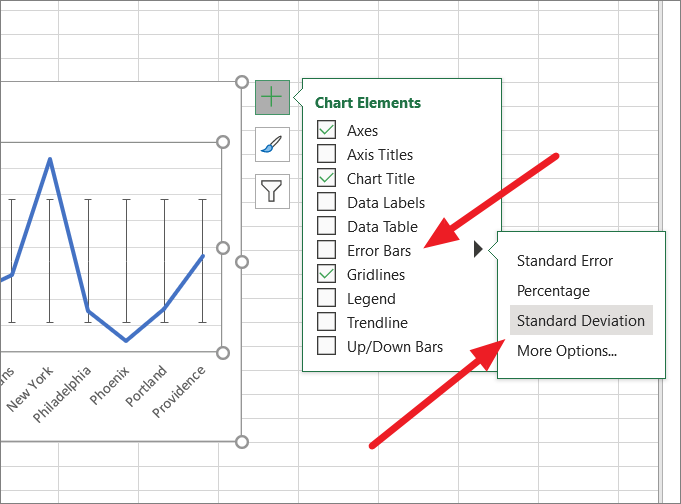
Then, click the ‘Error Bars’ option and select ‘Standard Deviation’.
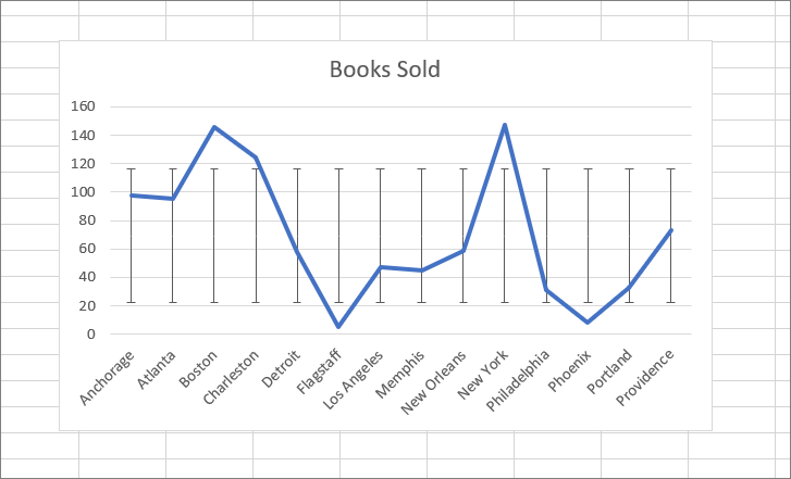
As a result, the standard deviation bars will be inserted for all data points as shown below.
Calculating Variance in Excel
When calculating the standard deviation of your data, you often need to calculate variance as well. Variance is the variability in the data which is also the square of the standard deviation. Similar to standard deviation, it also has 6 built-in functions that you can use to calculate the variance of your data. But, Microsoft recommends users to use VAR.S and VAR.P to calculate the variance of the sample data and population data respectively.
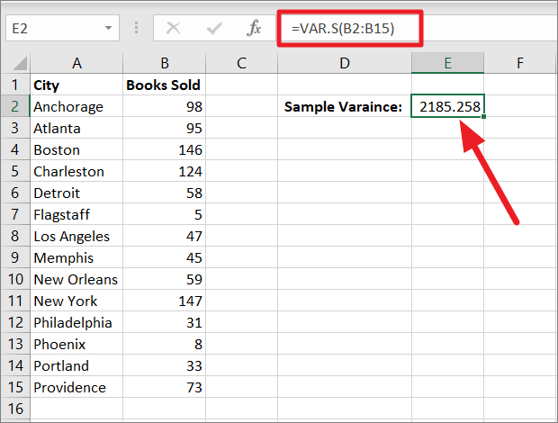
To calculates the variance based on the sample data, use the below formula:
=VAR.S(B2:B15)The above formula calculates sample variance for the range B2:B15 and displays the result in cell E2.
To calculates the variance based on the population data, use the below formula:
=VAR.P(B2:B15)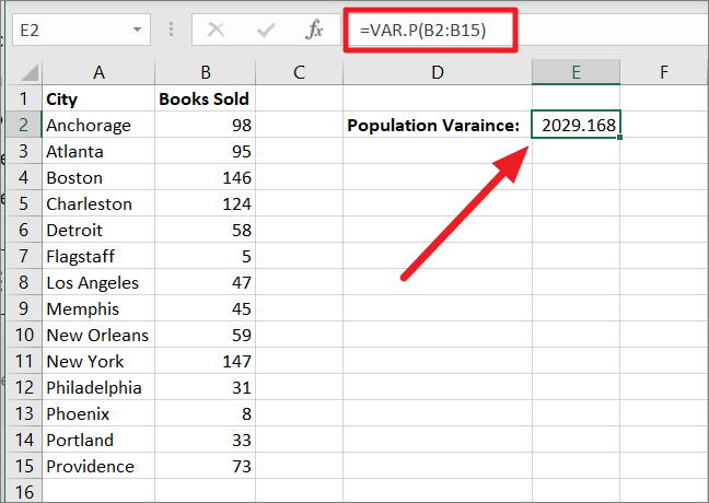
That’s it. That’s the only crash course you’ll ever need for calculating Standard Deviation in Excel. Now, go on and show off your newly acquired skills!


