
Google Sheets provides an easy way to temporarily hide rows or columns containing sensitive or unnecessary data without removing them. This feature allows you to focus on the most relevant information in your worksheet, especially when dealing with extensive datasets.
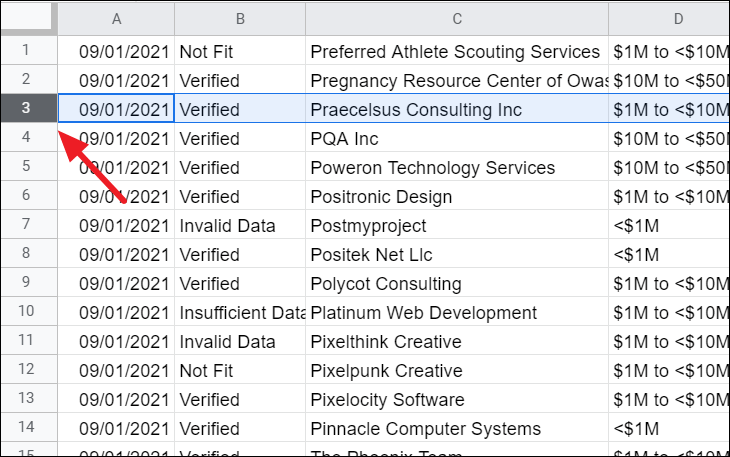
Hiding a single row or column in Google Sheets

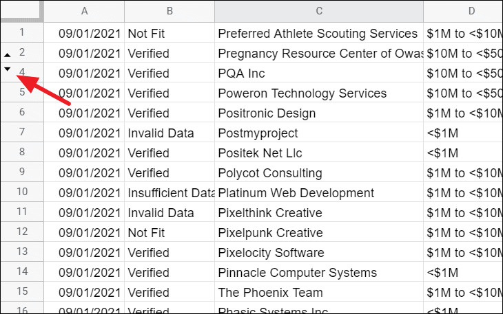
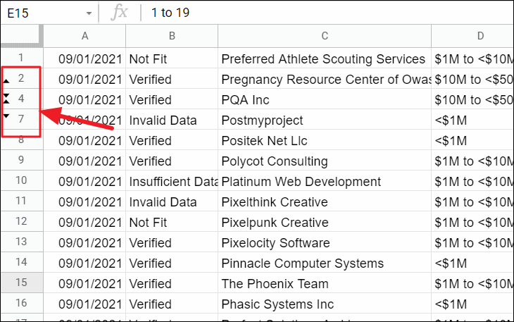
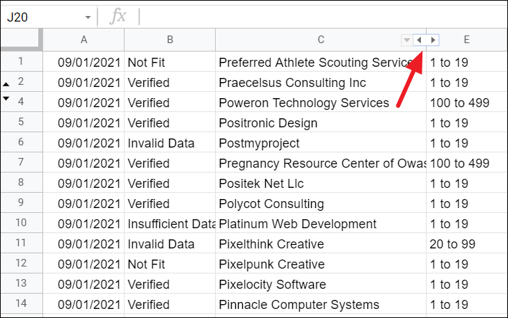
The selected row will now be hidden. You will notice arrow indicators between the adjacent row numbers, signifying a hidden row.
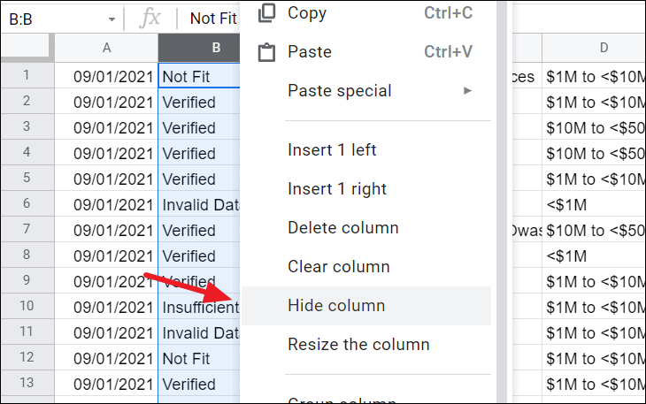
To hide a column, the process is similar.
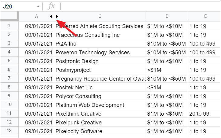
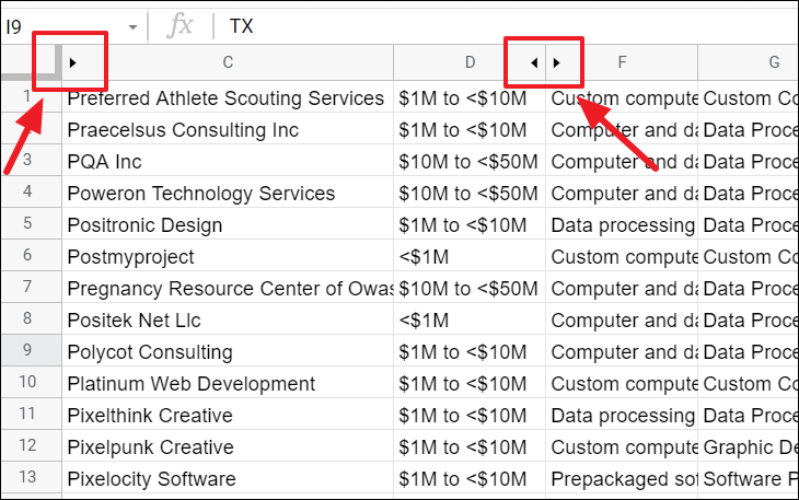
The column will now be hidden, indicated by arrow icons between the column headers.
Hiding multiple rows or columns in Google Sheets
To hide multiple rows, whether they are adjacent or non-adjacent, follow these steps:
Ctrl key and click on the row numbers you wish to hide. For example, to hide rows 3, 5, and 6, hold Ctrl and click on their row numbers.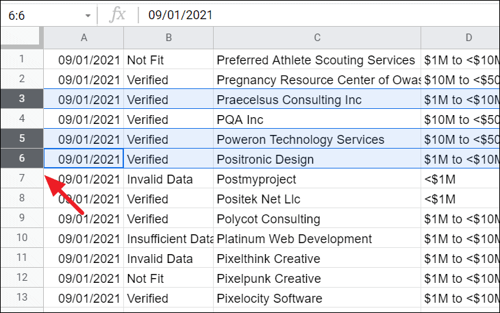
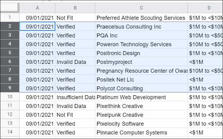
For adjacent rows, click and drag to select the range of rows, or click the first row number, hold down the Shift key, and click the last row number in the range. For example, to select rows 2 through 9, click on row 2, hold Shift, and click on row 9.
To hide multiple columns, use the same method as hiding multiple rows. Select the columns you wish to hide, either by holding down Ctrl to select non-adjacent columns or Shift for adjacent columns, and then right-click and choose Hide columns.
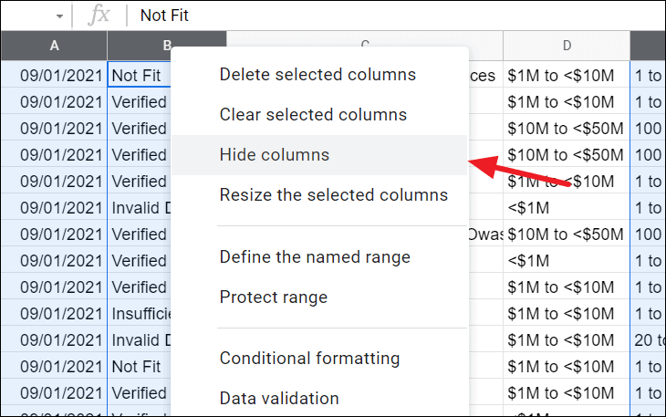
The selected columns will now be hidden from view.
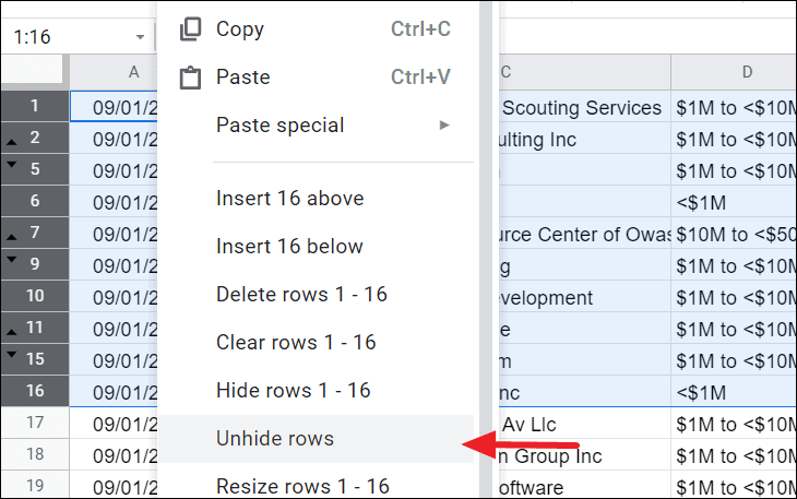
Unhiding a single row or column in Google Sheets
To unhide a hidden row or column, look for the arrow indicators between the row numbers or column letters. These arrows signify that there is a hidden row or column in that location.
The hidden row or column will become visible again, highlighted to indicate it has been unhidden.
You can use the same method to unhide rows by clicking on the corresponding arrow indicator.
Unhiding multiple rows or columns in Google Sheets
When dealing with multiple hidden rows or columns, especially in large spreadsheets, you can unhide them all at once.
Shift key, and click on the row number below the last hidden row.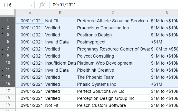
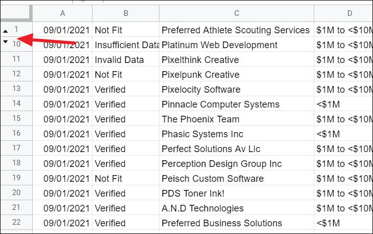
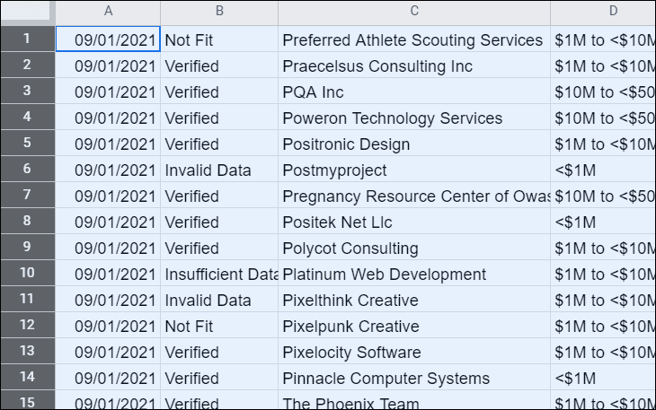
All hidden rows within the selected range will now be visible.
To unhide multiple columns, follow a similar process. Select the columns around the hidden ones by clicking on the column letter before the first hidden column, holding down the Shift key, and clicking on the column letter after the last hidden column.
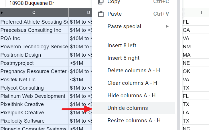
The hidden columns will now appear in your spreadsheet.
Hiding and unhiding rows or columns in Google Sheets is a straightforward process that helps manage and organize data effectively without deleting any information.