
Duplicate data in Google Sheets can cause confusion and inaccuracies in your spreadsheets. Identifying and highlighting these duplicates is essential for maintaining data integrity and ensuring accurate analysis.
Highlighting Entire Rows with Duplicate Data
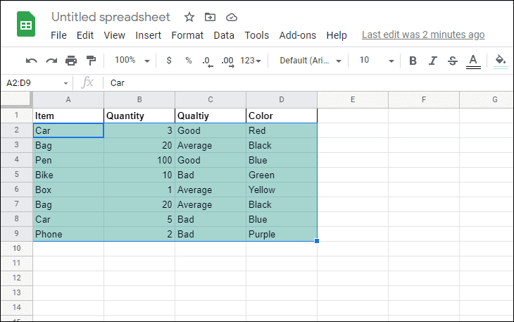
When working with extensive spreadsheets that contain interconnected data across multiple columns, it’s often more effective to highlight entire rows that contain duplicate values in a specific column. This ensures that any duplicate entries are easily noticeable, even if the duplicate cell is not currently visible on your screen.
Add another rule at the bottom.Apply to range field displays the correct range of cells you’ve selected. Under the Format cells if section, select Custom formula is from the dropdown menu.=countif($A$2:$A$9,$A2)>1This formula checks for duplicate values in column A. The dollar signs ($) ensure that the formula references the correct column and rows absolutely.
Formatting style section. Then, click Done to apply the rule.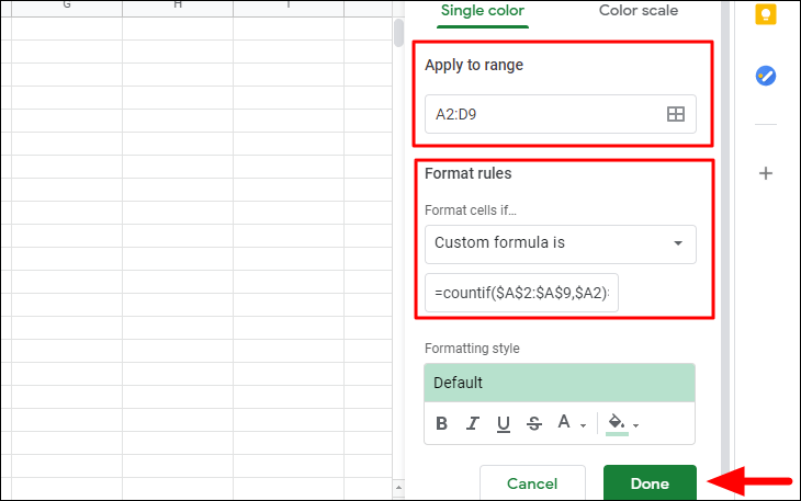
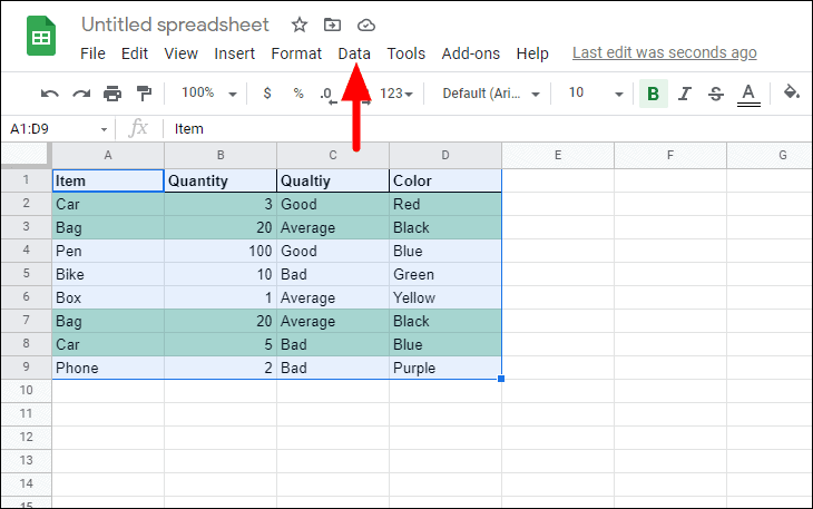
The entire rows containing duplicate entries in column A are now highlighted, making them easy to spot.
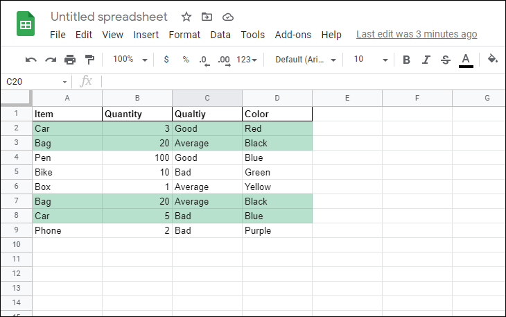
You can adjust the formula to check for duplicates in other columns by replacing $A$2:$A$9 and $A2 with the appropriate column references.
Highlighting Duplicate Cells in a Column
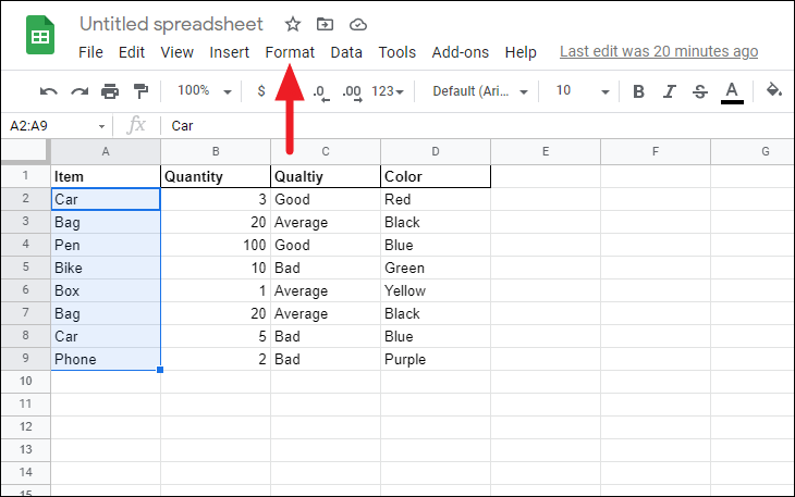
If you prefer to highlight only the duplicate cells within a specific column, you can achieve this using conditional formatting as well. This method is useful when you need to focus on duplicates in a single column without highlighting entire rows.
Apply to range field reflects the correct cells selected. Under the Format cells if section, choose Custom formula is from the dropdown menu.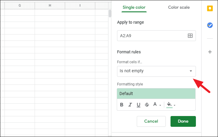
=countif($A$2:$A$9,A2)>1This formula counts how many times each value appears in the range and highlights the cells where the count is greater than one.
Done to apply the conditional formatting rule.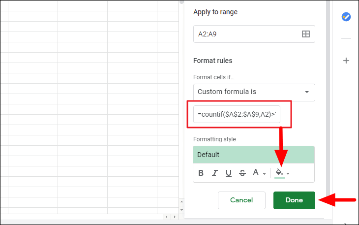
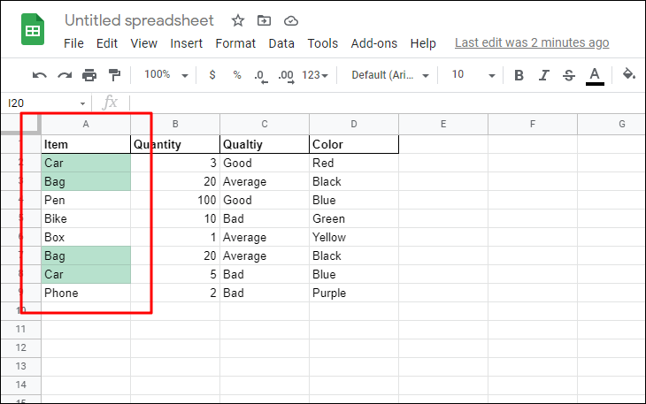
The duplicate cells within the selected column are now highlighted with the formatting you chose.
Removing Duplicate Data in Google Sheets
If you need to eliminate duplicate entries entirely, Google Sheets provides a built-in feature to remove them quickly. This method is efficient for cleaning up your data without manually deleting each duplicate row or cell.
Select all to consider entire rows or tick specific columns to check for duplicate values in those columns.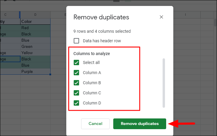
Remove duplicates at the bottom of the dialog box. Google Sheets will process the data and inform you of how many duplicate rows were removed and how many unique rows remain.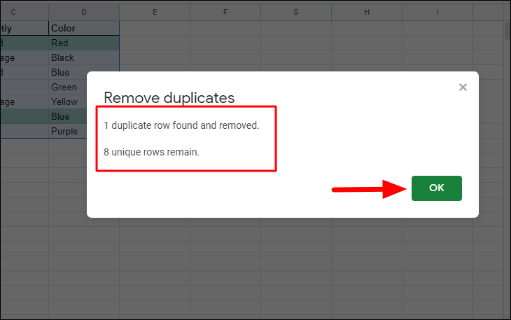
The duplicate data has now been removed from your selected range, streamlining your spreadsheet.
By effectively highlighting or removing duplicate data in Google Sheets, you can maintain clean and accurate spreadsheets. Utilizing these methods saves time and reduces errors, allowing you to focus on analyzing unique data entries.