Page Breaks are light grey lines or dotted lines that split or divide a worksheet into separate pages for printing. It splits the worksheet and shows you how much data is to be printed on a single page and then how much on the next page and so on. In other words, it marks the edges of each page.
There are two types of page breaks in Excel – manual page breaks (solid lines) and automatic page breaks (dashed lines). In the normal view of the worksheet, they will appear as horizontal and vertical lines. You can manually add page breaks to control where the data should break and continue to the next page, or Excel will automatically add page breaks when you check your worksheet in ‘Print Preview’ or ‘Page Break Preview’.
If you don’t plan on printing the worksheet or clearing the document of visual clutter, you can easily remove page breaks from an Excel document. In this post, we provide step-by-step instructions on how to insert, adjust, view, hide, and remove page breaks in Excel.
Insert Page Breaks in Excel
Excel automatically inserts page breaks according to paper dimensions and scale while printing an Excel spreadsheet. You can identify automatic page breakers by their dotted or dashed line along the lines of the cell border.
However, sometimes you may want to manually insert page breakers if you don’t like the way Excel assigned page breaks or if you only want specific columns/rows of data on each printing page. There are two kinds of page breaks – vertical and horizontal. On a spreadsheet, you can insert vertical page breaks, horizontal page breaks, or both. Here’s how to insert manual page breaks in excel.
Insert Vertical Page Breaks in Excel
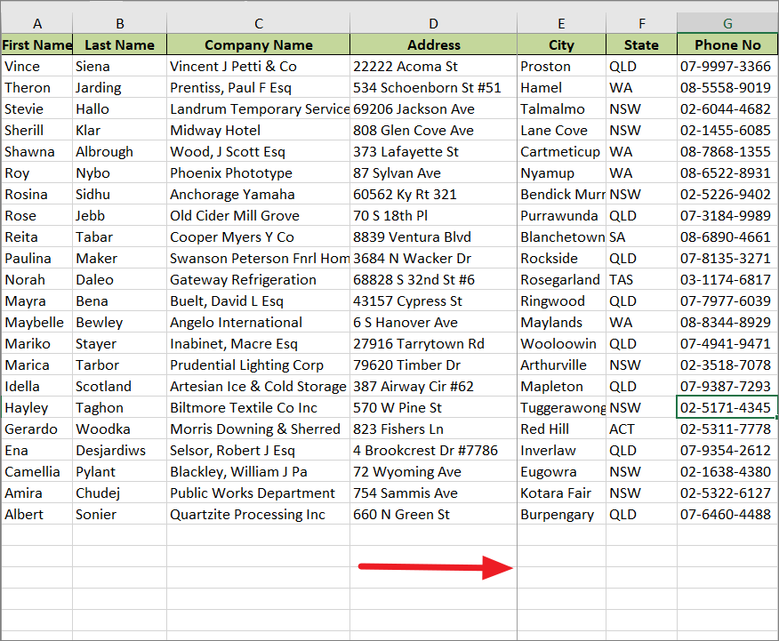
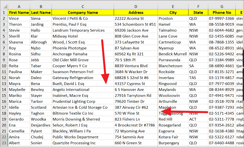
Suppose, you have a list of employee details in several columns such as First Name, Last Name, Company Name, Address, City, State, Phone number, Email, etc. If you try to print the worksheet, at least the first 6 columns will be printed on the same page. But you only want to print the first four columns (First Name, Last Name, Company Name Address) on the first page and the rest on the next page. This can be done by inserting a vertical page break between the fourth and fifth columns.
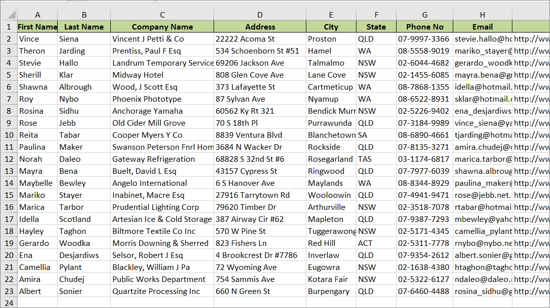
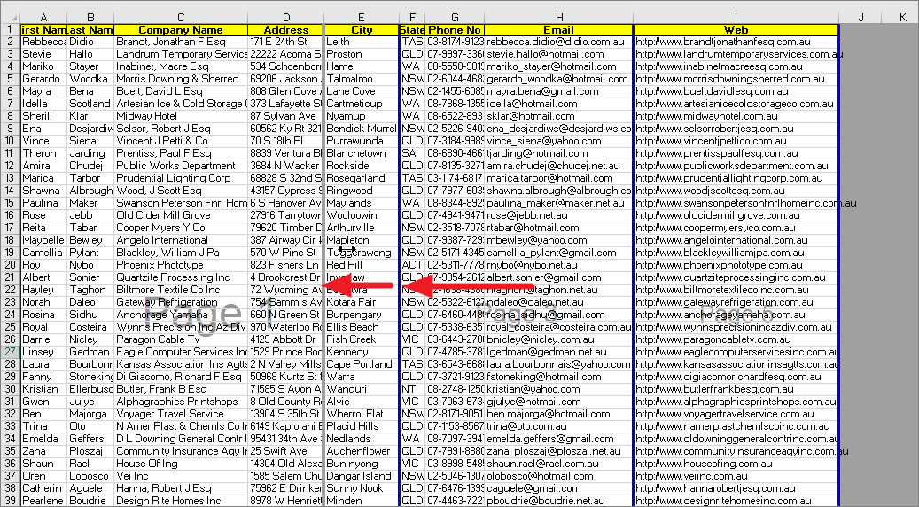
First, select the column to the right of where you want to insert the page break. We need to insert a page break between columns D and E, so we selected column E. To select the whole column, simply click the column letter E.
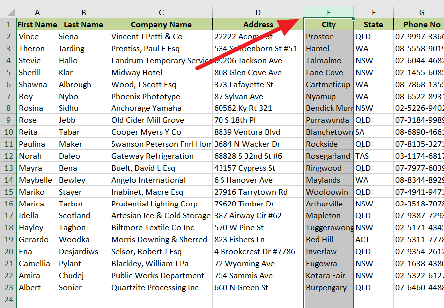
After that, go to the ‘Page Layout’ tab and click the ‘Breaks’ drop-down arrow in the Page Setup section. Then, select the ‘Insert Page Break’ option. Alternatively, you can also insert page breaks by pressing the keyboard shortcut Alt + P + B + I.
Once you do that, Excel will divide the page and insert a page to the left of the selected cell. The page break line will be slightly darker than cell gridlines as shown below.
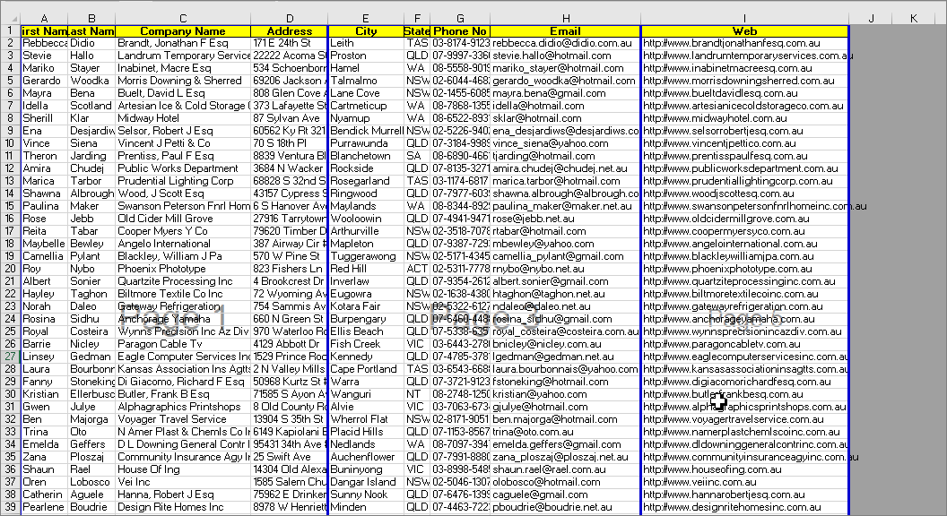
The page breaks are only slightly darker than the gridlines, so if they are not clearly visible, you can remove the cell gridlines to see them properly. To remove the gridlines, go to the ‘View’ tab and uncheck the ‘Gridlines’ option in the Show group.
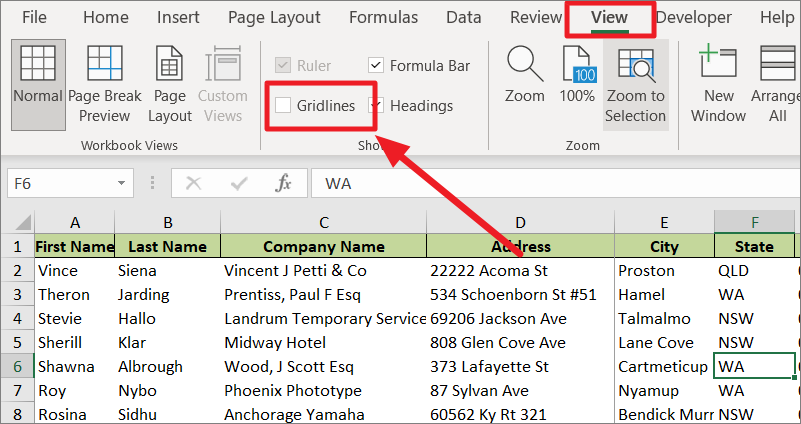
This will remove all the cell’s gridlines leaving only the page break behind.
Insert Horizontal Page Breaks in Excel
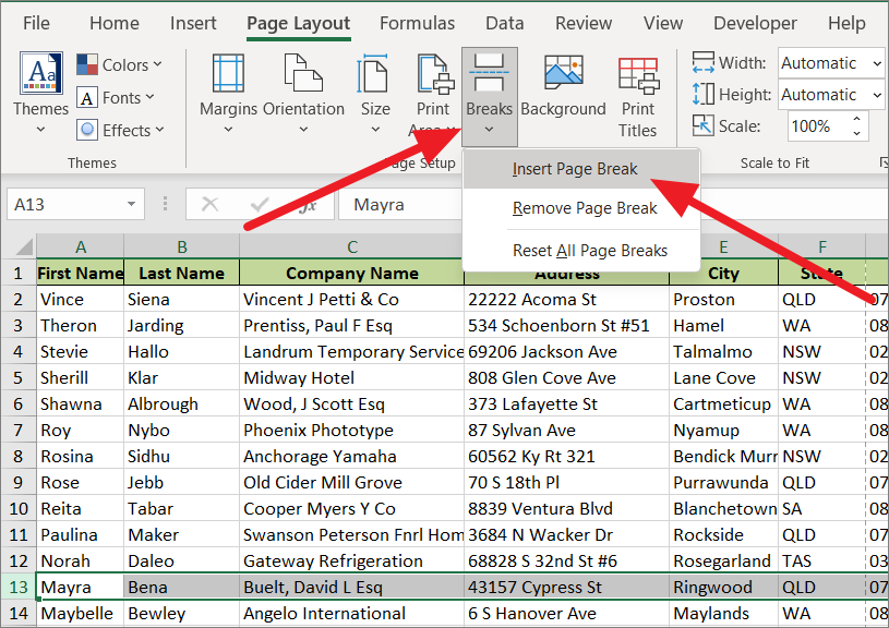
Let’s assume we have a list of employee information in a spreadsheet, but we only want to print 11 employees’ details on a page. To do this, we need to insert a page break between rows 12 and 13 (because the top row is with headers). You can use similar steps to insert page breaks between rows.
First, select the row that is just below where you want the page break to appear. In contrast to the column where the page break appears to the right of the selected column, the page break appears above the selected row. Make sure to select the entire row by clicking on the row number. We need to insert the page break between rows 12 and 13, so we selected row 13.
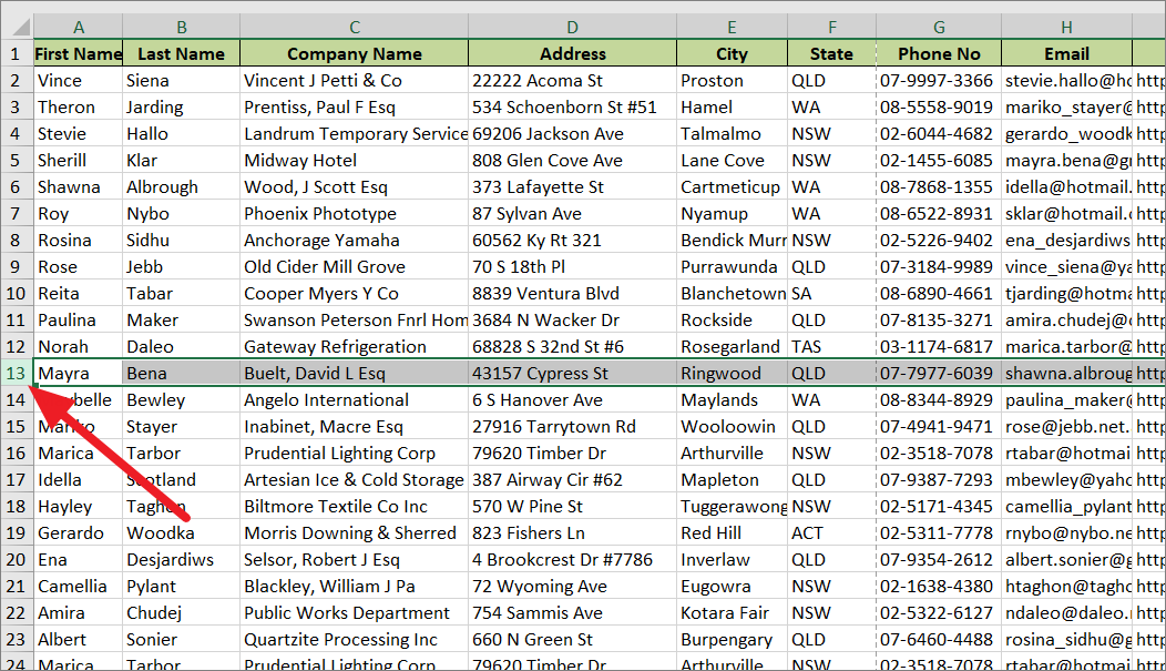
Then, head to the ‘Page Layout’ tab and click the ‘Breaks’ drop-down arrow in the Page Setup section. Then, select the ‘Insert Page Break’ option. Alternatively, you can also insert page breaks by pressing the keyboard shortcut Alt + P + B + I.
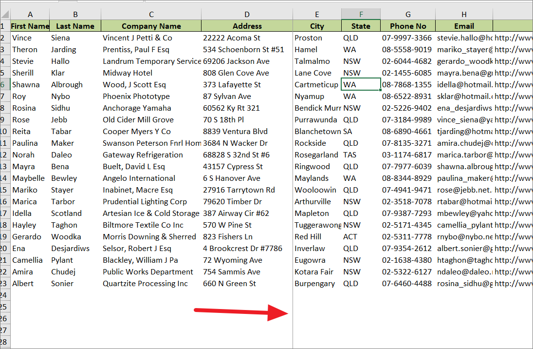
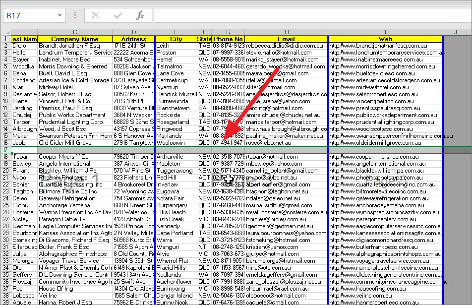
Once you click the ‘Insert Page Break’ option, you will see page breaks in a slightly darker gray line as shown below.
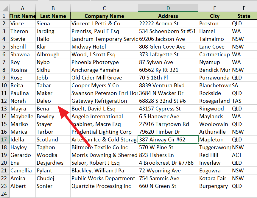
If the page break is not visible clearly, you can remove the gridlines to see them.
Insert Both Horizontal and Vertical Page Breaks Simultaneously
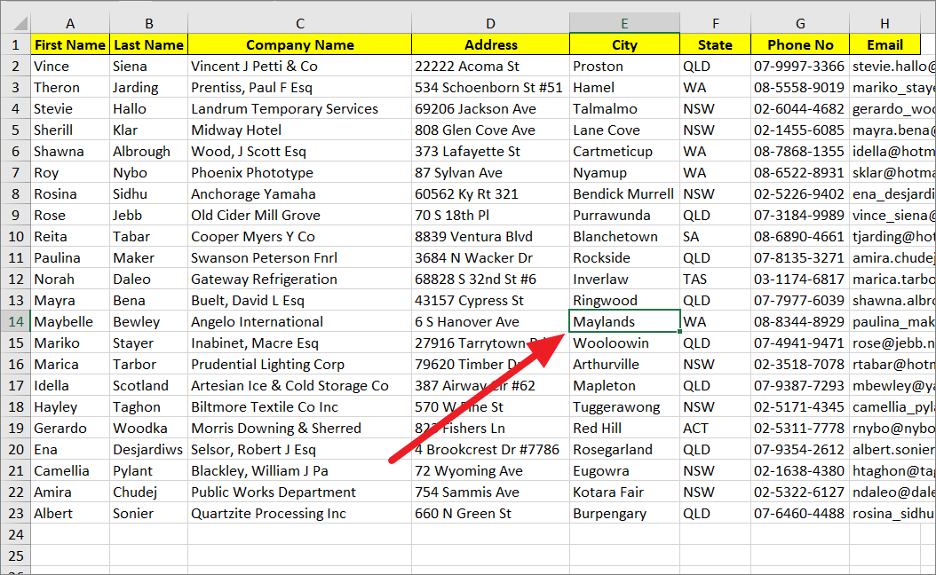
Besides vertical and horizontal page breaks, you can also add a crisscross page break at a specific location in your spreadsheet. To insert horizontal and vertical page breaks simultaneously, you have to select a cell instead of a whole row or column.
First, select the cell that is just below where you want the horizontal page break and to the right of where you want to insert the vertical page break. So, we selected cell E14 in the below example. The horizontal and vertical page breaks will intersect at the top left corner of the selected cell.
Then, use similar steps to insert page breaks. Switch to the ‘Page Layout’ tab, click the ‘Breaks’ drop-down menu, and select the ‘Insert Page Break’ option.
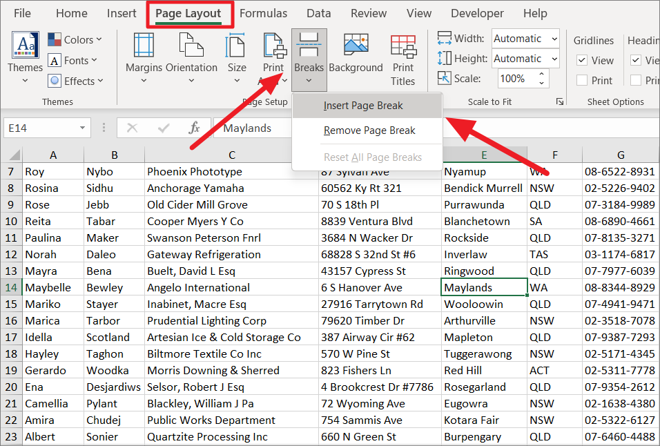
This will add horizontal and vertical page breaks, which is a cross line to the left and above the selection as shown below.
See/View Page Breaks in Excel
Page Break is a grey line that is slightly darker than the gridlines. Sometimes it is difficult to notice page breaks, especially on a spreadsheet full of data. To move, adjust, or remove page breaks, first, you need to see them. To view or adjust the page breaks, you need to enable the ‘Page Break Preview’ mode. The Page Break Preview is also helpful when you want to see how any changes you make (formatting or page orientation) affect the page breaks, automatic or manual.
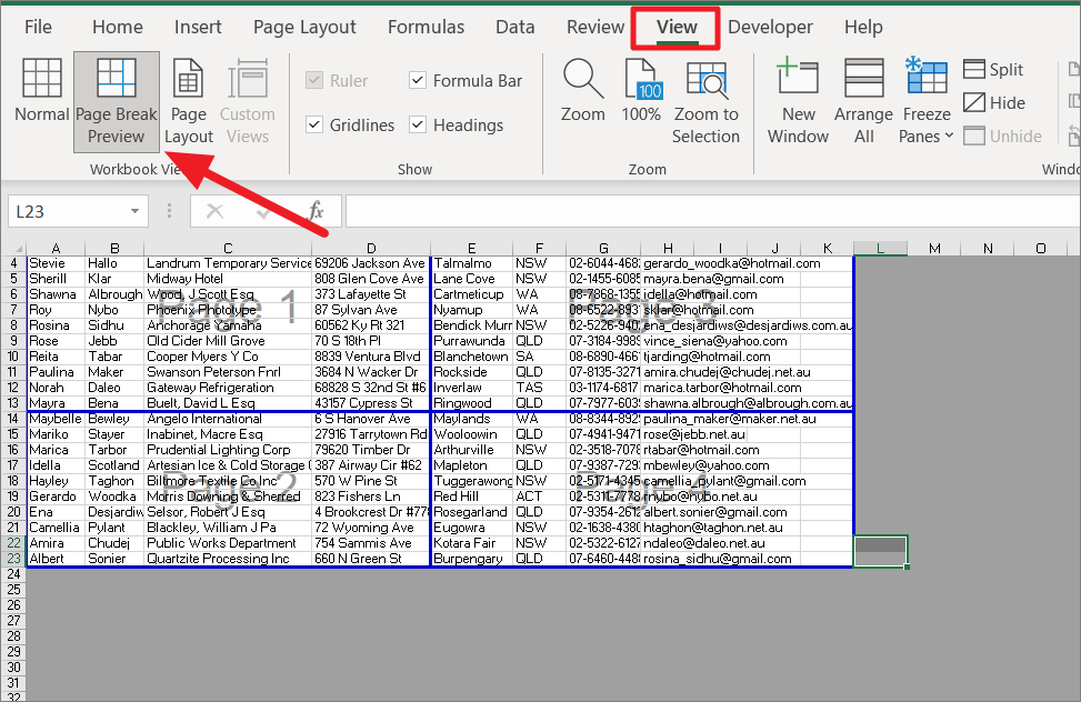
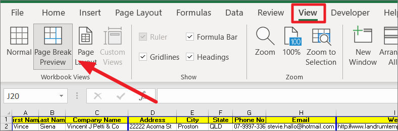
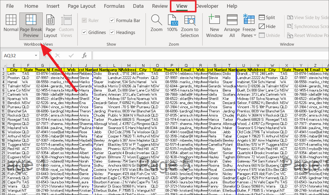
Open the spreadsheet and go to the ‘View’ tab on the ribbon. Then, click the ‘Page Break Preview’ option in the Workbook Views group.
Now, you will see all the page breaks and pages in the worksheet. You can also get the preview of the page in the Print Preview window, however, it will only show you data of a single page.
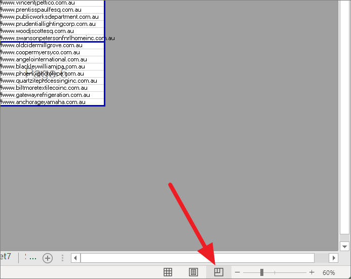
Alternatively, you can also use the Status bar to enable Page Break Preview in Excel. Click the rightmost icon next to the Zoom controls to view the ‘Page Break Preview’. You can also use the keyboard shortcut Alt+Win.
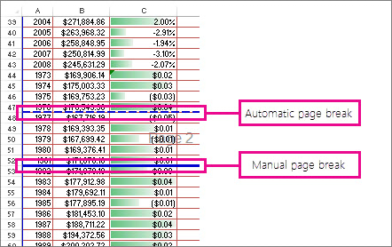
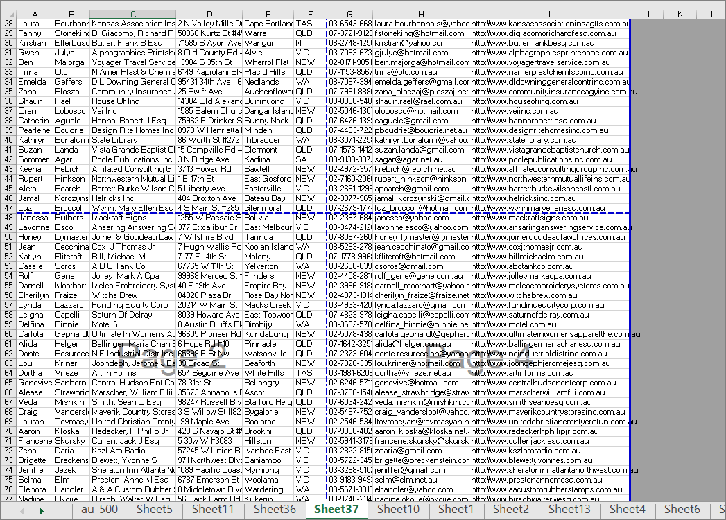
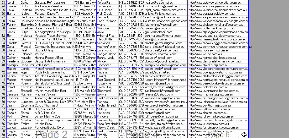
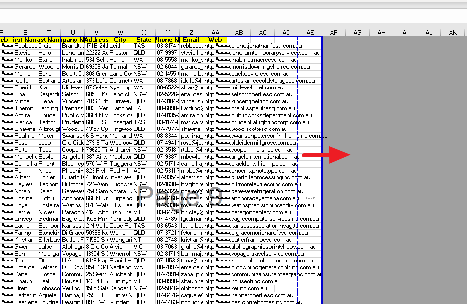
As you can see below, the page breaks will appear in blue lines and the split pages will be numbered.
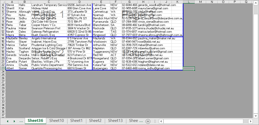
And the Zoom level of the page will automatically reduce to 60% to show as many pages break as possible. You can also adjust the zoom level to your desired level.
The automatic page breaks (if there are any) will be shown as dashed lines and the manual page breaks will appear as solid lines.
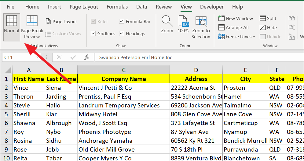
To go back to the normal view, click the ‘Normal View’ button in the ribbon.
Move Page Breaks in Excel
After inserting the page breaks in the worksheet, you can manually move them to your desired place. You can move horizontal or vertical page breaks by dragging them to another location. Also, page break cannot be moved to the middle of the cells, it can only be moved from gridlines to gridlines (cell border).
Move a Manual Page Break
To adjust a page break, first, you need to be in Page Break View mode. Go to the ‘View’ tab on the Ribbon and click the ‘Page Break Preview’ button or click on the ‘Page Break Preview’ icon on the Status Bar.
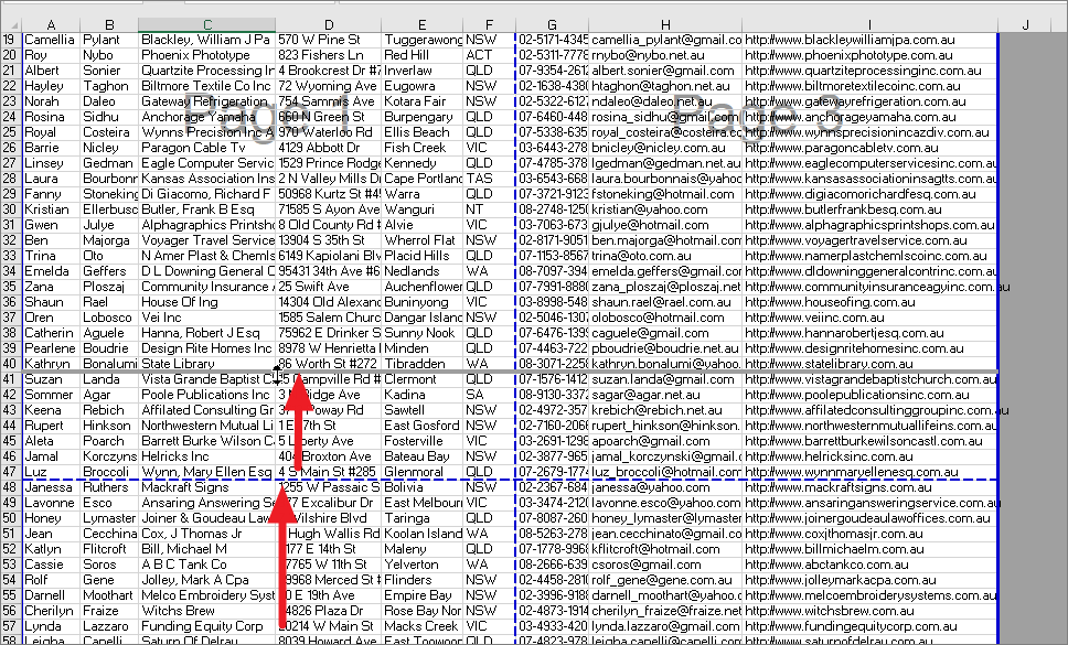
Then, hover your cursor over the page break you want to move. Once you do that, the cursor will change into a double-edged arrow indicating the direction in which the page break can be moved.
Now, you can click and drag the blue-colored page break to your desired location.
The page break is moved from between columns D and E to between columns C and D.
Move an Automatic Page Break
Similar to manual page breaks, automatic page breaks can also be moved to another location. But once moved, an automatic page break will become a manual page break. You can easily spot automatic page breaks with their dashed lines.
First, you need to view the worksheet in ‘page break preview’.
Then, hover over the automatic page break (dashed lines) you want to move and drag the double-headed arrow to where you want it to be placed.
Once moved automatic page break will change into a manual page break, i.e., the dashed blue line will change into a solid blue line.
Hide or Show Page Breaks Marks
Once the page breaks are added, they would not disappear until you save and reopen the document. If you don’t want page breaks to be visible on the worksheet, you can hide them anytime. Here’s how you can hide or show page break marks in Excel:
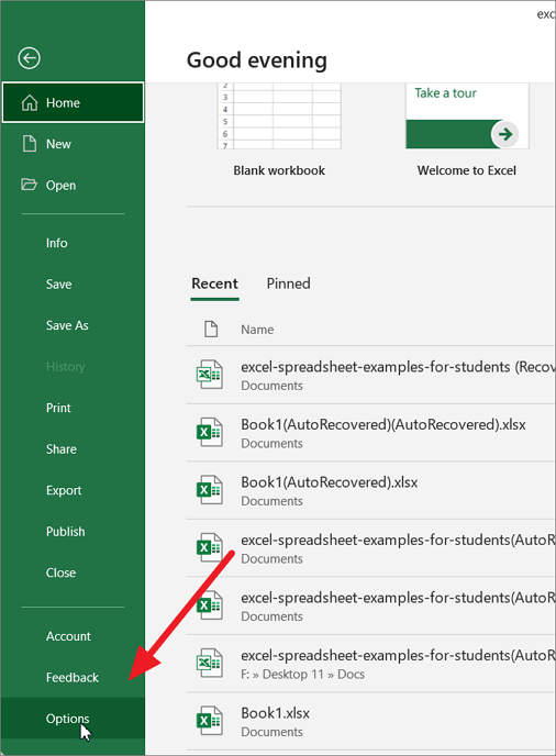
Open the ‘File’ menu and click ‘Options’ in the Excel backstage view.
In the Excel Options window, select ‘Advanced’ from the left pane and then scroll down to the ‘Display options for this worksheet’ section on the right. Then, uncheck the ‘Show page break’ checkbox. After that, click ‘OK’ to apply the changes.
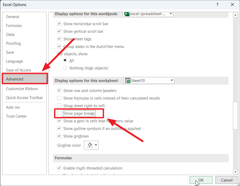
Note: Make sure, you are in the ‘Normal’ view and not in ‘Page Break Preview’. Otherwise, the above option would not be unavailable.
The above steps will only hide page breaks for the current workbook. If you want to hide page breaks on other workbooks, you must follow the same steps for every workbook.
Remove Page Breaks in Excel
If you don’t like the page breaks on your workbook, you can easily remove them. Although, removing or deleting manual page breaks in Excel is easy, removing automatic page breaks is a bit tricky. You can remove a single page break at a time (horizontal or vertical), vertical and horizontal page breaks at the same time (crisscross page breaks) or all the page breaks at once.
Remove the Manually Inserted Horizontal Page Breaks
If you have manually inserted horizontal page breaks, you can easily remove or delete them with these steps:
First, open the spreadsheet in which you want to remove horizontal page breaks. Then, head to the ‘View’ tab and select the ‘Page Break Preview’ option to turn every page break visible.
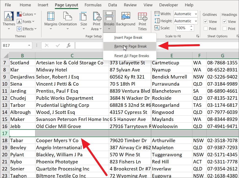
Next, select the row just beneath the page break that you want to remove.
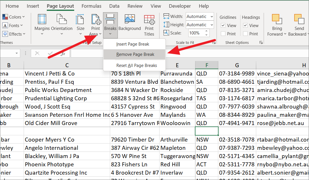
After selecting the row, go to the ‘Page Layout’ tab, then click the ‘Breaks’ button and select ‘Remove Page Break’.
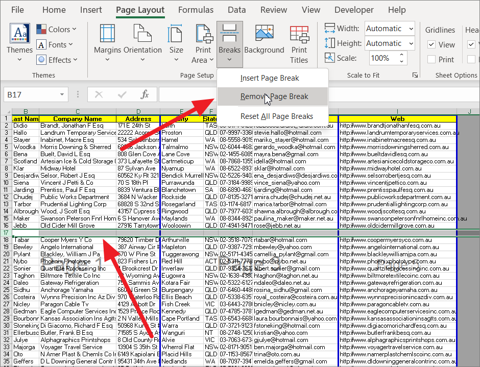
Alternatively, you can just select the appropriate row and then go to the ‘Page Layout’ tab, click the ‘Breaks’ button and select ‘Remove Page Break’.
Remove Manually Inserted Vertical Page Breaks
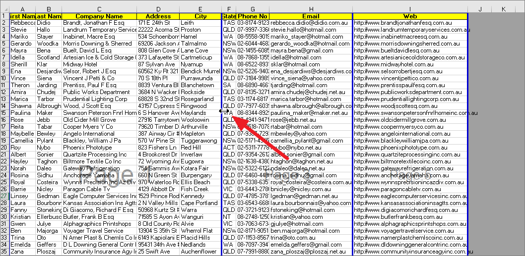
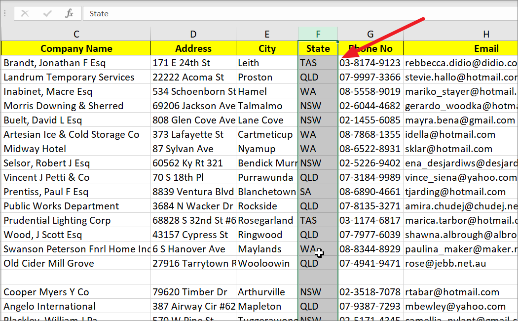
If you want to remove vertical page breaks, you need to select the column to the right of the page break.
First, view the spreadsheet in the page break preview. To remove a vertical page break, select the column to the right of the page break that you want to delete.
Next, click the ‘Breaks’ menu and select ‘Remove Page Break’ under the ‘Page Layout’ tab.
Now, you will notice that the vertical page break has been deleted.
Remove Vertical and Horizontal Page Breaks at Once (Crisscross Page Break)
We have seen how to insert vertical and horizontal page breaks at the same time. We can also remove the two page breaks (vertical and horizontal) at once. To remove the two page breaks at the same time, you have to select a cell where both vertical and horizontal page breaks intersect. Let’s see how to remove both vertical and horizontal page breaks at once:
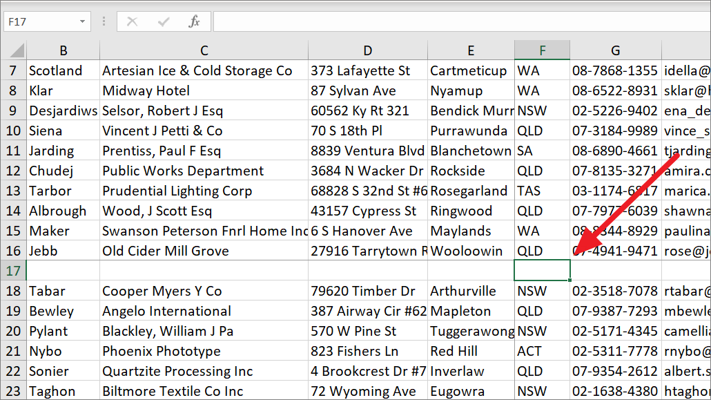
For example, we want to remove the page breaks at column F and row 17. To remove this crisscross page break, first, open the spreadsheet. You can also get into Page Break Preview mode to easily spot the page break lines.
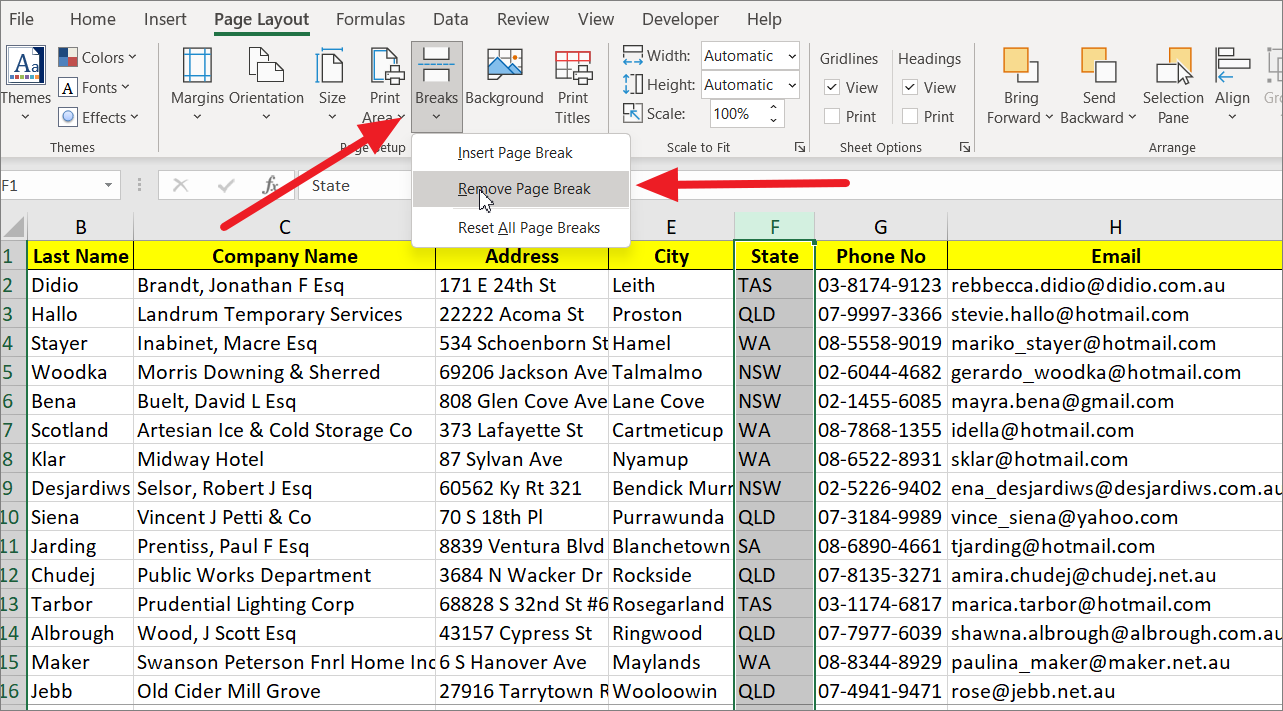
Next, select the cell to right and below where both vertical and horizontal page break grey lines meet. In this example, it’s cell F17.
After that, navigate to the ‘Page Layout’ tab in the Excel ribbon, click the ‘Breaks’ menu in the Page Setup group and then select ‘Remove Page Break’.
You will see both vertical and horizontal page breaks have been removed at once.
Reset all Manual Page Breaks
Excel only has options to remove manual page breaks but not automatic page breaks. If you don’t have time to remove page breaks one by one, you can reset all page breaks which will remove all manual page breaks from the current worksheet. However, if the worksheet has automatic page breaks, they will remain in the worksheet.
Open the spreadsheet where you want to reset all page breaks and switch to page break preview mode.
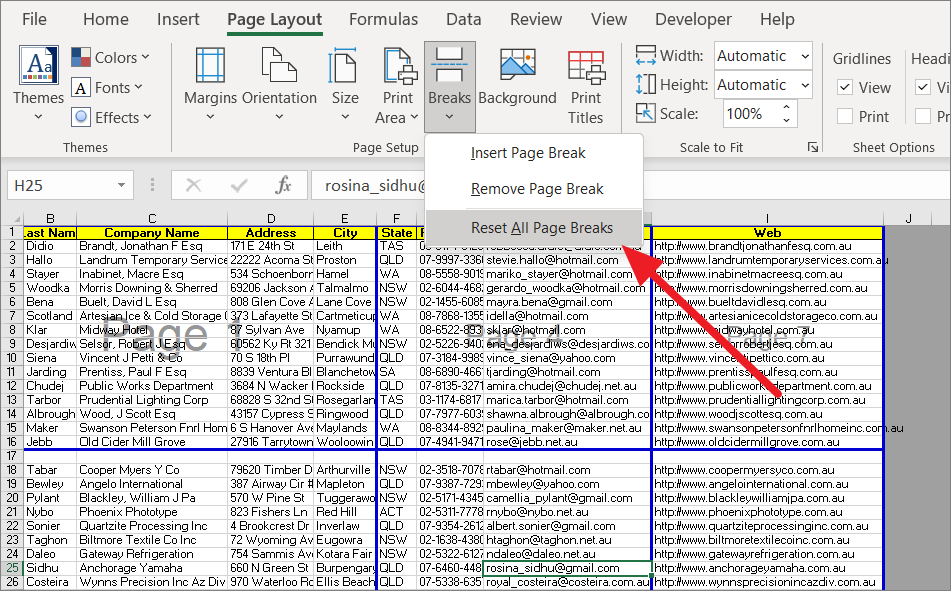
Next, go to the ‘Page Layout’ tab in the Page Setup group and click ‘Breaks’. Then, select the ‘Reset All Page Breaks’ option from the drop-down menu.
This will delete all page breaks from the worksheet.
How to Remove Automatic Page Breaks in Excel
Excel automatically inserts page breaks (dashed lines) while printing or when you switch to Page Break Preview mode based on page size, margin, scale, and position of other manual page break lines you inserted. Automatic Page Breaks cannot be removed with the ‘Remove Page Breaks’ or ‘Reset All Page Breaks’ option. There are two ways to remove automatic page breaks in Excel: using VBA code or using the drag and drop method.
Use VBA Code to Remove any Page Breaks in Excel
You can apply a simple VBA script to remove any page breaks in Excel. Follow these steps to apply the VBA code:
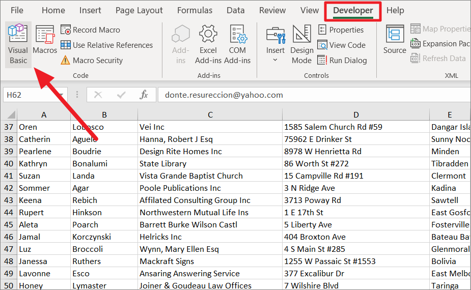
First, open the workbook where you want to remove automatic page breaks, manual page breaks, or both. Then, go to the ‘Developer’ tab and click the ‘Visual Basic’ option from the ribbon or press Alt+F11 to open Microsoft Visual Basic for Applications.
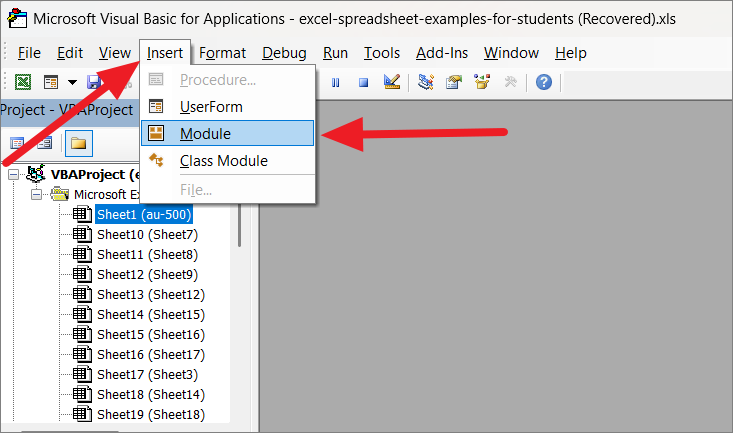
This will open Microsoft Visual Basic for Applications in a separate window. In the VBA window, click the ‘Insert’ menu, and select the ‘Module’. Alternatively, you can just right-click on the ‘Microsoft Excel Objects’ in the navigation bar on the left, click ‘Insert’, and then select ‘Module’ from the sub-menu.
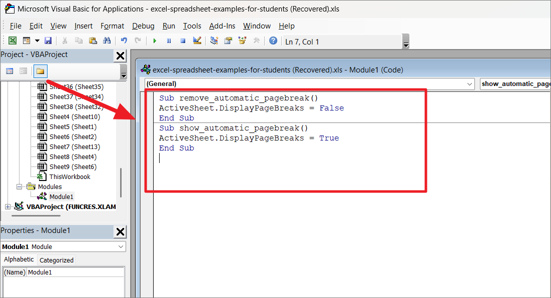
Now, copy and paste the following VBA script into the new module window:
Sub remove_automatic_pagebreak()
ActiveSheet.DisplayPageBreaks = False
End Sub
Sub show_automatic_pagebreak()
ActiveSheet.DisplayPageBreaks = True
End Sub
The above code allows you to remove page breaks or show page breaks again.
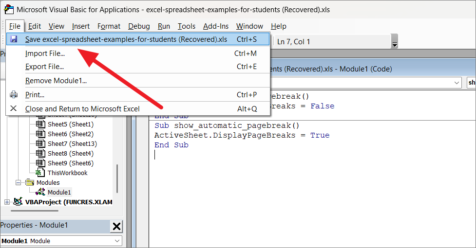
After pasting the script, click ‘File’ and select ‘Save XXXX (filename)’ to save this module as a macro.
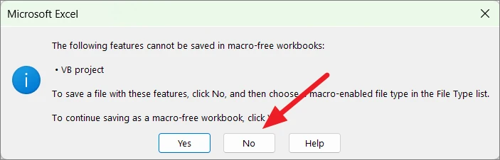
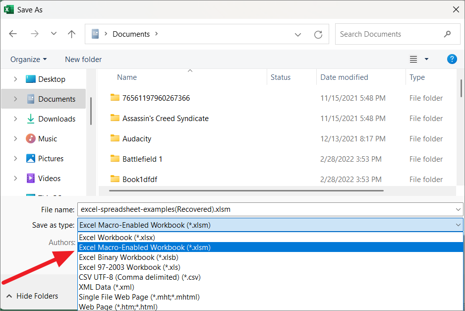
The VB script needs to be saved in a macro-enabled file type. Once you click Save, you will see a prompt box asking whether you want to save this file in a macro-free file or macro-enabled file type.
Click ‘No’ to choose the macro-enabled file type.
In the Save As window, choose ‘Excel Macro-Enabled Workbook (*.xlsm)’ format from the ‘Save As type’ drop-down and then click ‘Save’.
Now, you can run the macro to remove or show page breaks.
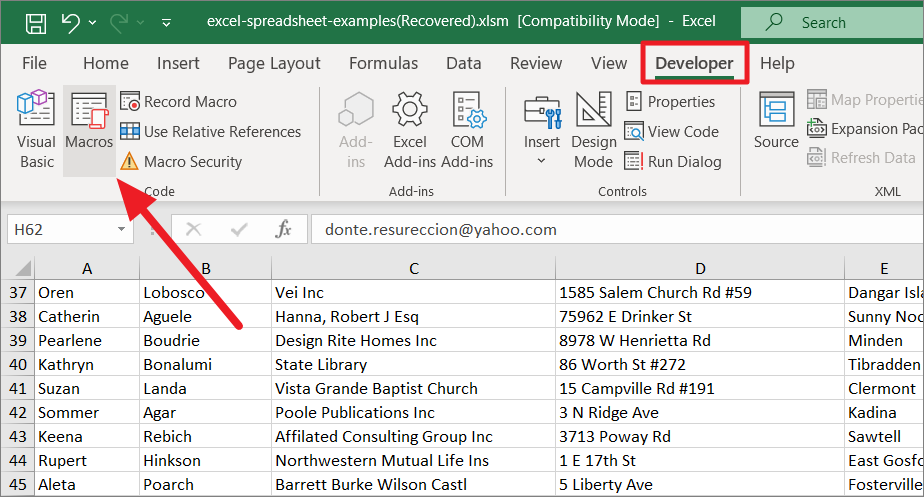
Go back to your Excel worksheet, then head to the ‘Developer’ tab in ‘Ribbon’ and select ‘Macros’ or press ALT+F8.
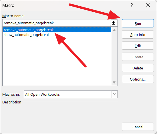
A dialog box named Macro will open up. Under the Macro name, you will see two macro names. Now, select ‘remove_automatic_pagebreak’ macro and click ‘Run’.
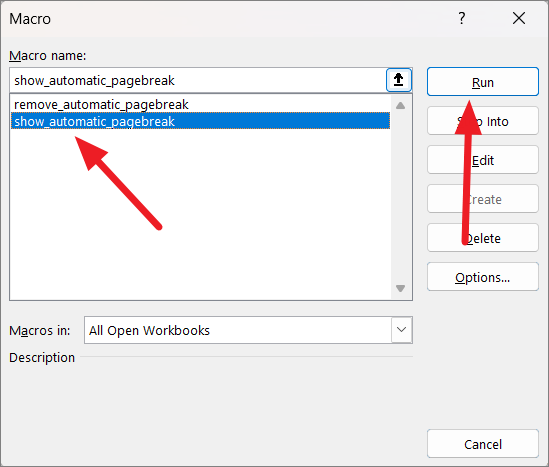
To show all the page breaks again, open the macro window again, select the ‘show_automatic_pagebreak’ macro and click ‘Run’.
Use Drag and Drop Option to Remove Manual Page Break
Another way to remove automatic page breaks is to use the drag and drop method to hide or remove automatic page breaks. You can also drag the automatic page break to a new location to change it to a manual page break then use the above method to delete the page break.
First, go to the ‘View’ tab in Ribbon and select ‘Page Break Preview’ to view the spreadsheet in page break preview mode.
Once we are in Page Break Preview, click the automatic page break line you want to remove and drag it across the last border, and the page break line will be disappeared.
When you remove a vertical or horizontal page break, another vertical or horizontal line perpendicular to the deleted line will also be disappeared. Repeat the steps to remove as many automatic page breaks as you want.
Alternatively, you can also drag the automatic page break to a new location, which will turn it into a manual page break. Then, use the ‘Remove Page Break’ option under ‘Breaks’ in the Page Layout tab to delete it.
That’s it. Now, you know everything there is to know about page breaks in Excel, from adding, adjusting, hiding, or removing them.