
If you have used SUMIF and COUNTIF in Excel, then another statistical categorical function that is important and useful to learn is the AVERAGEIF. Excel’s AVERAGEIF function calculates the average of the given values or numbers in a range of cells if the given values meet the criteria you specified.
Similar to SUMIF and COUNTIF, AVERAGEIF also has two versions of itself: AVERAGEIF and AVERAGEIFS. One is for handling single criteria and the other (AVERAGEIFS) is for handling more than one set of criteria. AVERAGEIF function is used for data analysis to calculate the mean of the given values based on the criteria.
For example, let’s assume you have a list of fruits that are sold in a shop and their prices throughout the month, and you want to calculate the average price of one of the fruits (e.g. Mangoes). You can use the AVERAGEIF function with Mangoes as the criteria and price list as the range of values to calculate the average price of only mangoes.
Calculate Average Based on a Single Criteria with AVERAGEIF Function
You can use the AVERAGEIF function in Excel to calculate the average for values in a single range of cells based on a single criterion.
Syntax and Arguments for the AVERAGEIF function:
=AVERAGEIF(range, criteria, [average_range])Arguments:
range(required) – The range of cells upon which the given criteria will be tested against to find the average (for the values in the corresponding cells). It can include numbers, arrays, or references that consist of numbers.- criteria (required) – The criterion that is compared against the range to determine which cells will be averaged. It can be number, expression, cell reference, or text.
- [average_range] (optional) – It is the actual range of cells that contains numbers that need to be averaged. If this argument is omitted in the formula, the given
rangeis used.
The criteria for the formula can be made up of number, date, expression (with logical formula), cell reference, text, a formula, or wildcards (*, ?) for partial matching. And number, date, text, and cell reference can also be combined with logical operators such as (<, >, <=,>=,<>, =) to form criteria.
Basic Example:
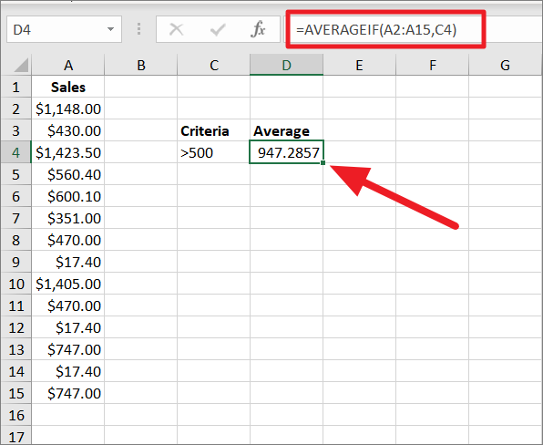
Lets us explain how this function works in a basic example before continuing to more complex examples. In the below dataset, we have a list of sales and we wish to average the values that are greater than 500. To do that, we can use the below formula:
=AVERAGEIF(A2:A15,">500")Since the range and average_range are the same in this sample data set, we omitted the last argument, but the formula automatically assumes A2:A15 as the average_range and calculates the average for values that are greater than 500 (>500).
Unless the criteria is a plain number or cell reference, you need to always enclose the criteria in double quotes. The below formula produces the same result as the above formula but we specified the cell that contains the criteria.
Numerical Criteria
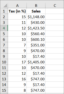
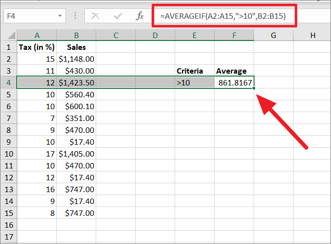
AVERAGEIF function was designed to check the criteria against one range or column and averages the values in a corresponding range, so it needs two columns to do that. Let’s assume you have the below the table with two columns and you want to calculate the conditional average for one column:
Use the below formula to calculate the average:
=AVERAGEIF(A2:A15,">10",B2:B15)The formula checks the range A2:A15 for values greater than 10% and if the values are found (to meet the criteria), it calculates the average for the corresponding values in the range B2:B15.
or, use this formula where the criterion argument is referenced to the cell that contains the criterion:
=AVERAGEIF(A2:A15,E4,B2:B15)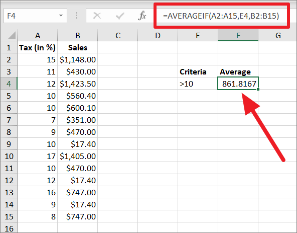
The logical or comparison operators can often be combined with numbers and dates to create criteria for the AVERAGEIF function. Here’s the list of logical operators you can use:
| Operator | Description | Example | Meaning |
|---|---|---|---|
| = | Equal to | “=500” | Equal to 500 |
| <> | Not equal to | “<>500″ | Not equal to 500 |
| > | Greater than | “>500” | Greater than 500 |
| < | Less than | “<500” | Less than 500 |
| >= | Greater than or equal to | “>=500” | Greater than or equal to 500 |
| <= | Less than or equal to | “<=500” | Less than or equal to 500 |
Text Criteria
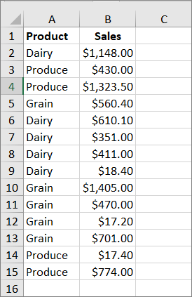
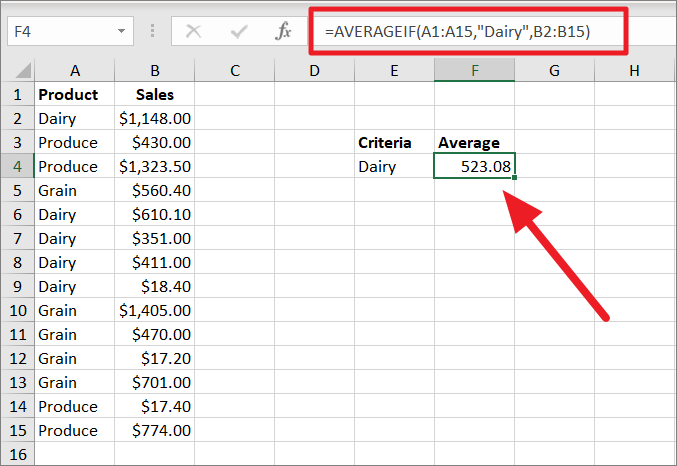
You often need to use text criteria to calculate the average for values that match the criteria. For example, the below data set contain a list of products and sales record.
To evaluate average sales of all dairy products, type the below formula:
=AVERAGEIF(A1:A14,"Dairy",B2:B15)The formula calculates the average for values in B2:B15 if the corresponding cells in the range A1:A15 has the exact value ‘Dairy’ (criteria).
Example 2:
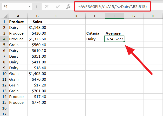
The text can also be combined with logical operators ‘not equal to’ (<>) or equal to (=) to get the average values.
To calculate the average sales for all products except the diary product, try the below formula.
=AVERAGEIF(A1:A15,"<>Dairy",B2:B15)The formula calculates the average of values in B2:B15 if the corresponding cells in the range A1:A15 are not ‘Dairy’ (<>Dairy).
Date Criteria
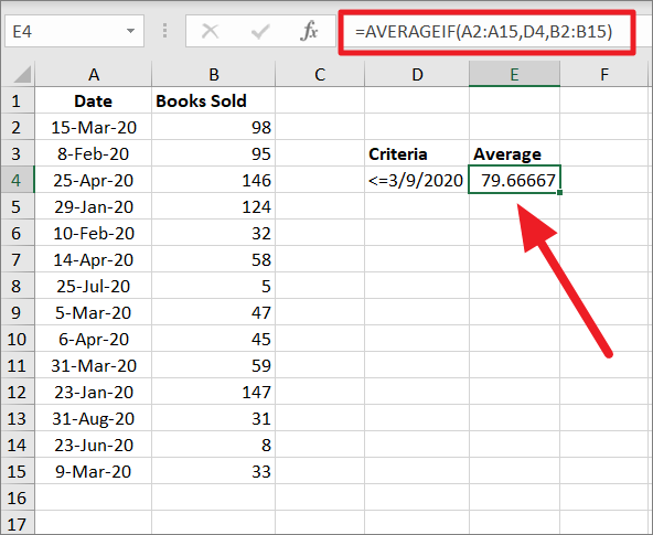
When working with the AVERAGEIF function, you can also use a date as criteria, similar to the numerical and text criteria. Let’s take a look at this table which contains the number of books sold on different dates.
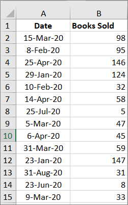
Now, with this formula, we can find the average of books sold on or before March 9:
=AVERAGEIF(A2:A15,D4,B2:B15)To specify the date condition ‘on or before March 9’, here, we are using <=March 9 (less than or equal to March 9) which is entered in the cell D4 and that cell reference is used as criteria instead. The formula looks up the range A2:A15 for the date March 9 or before March 9. If the condition is met, the formula evaluates the average for corresponding values in B2:B15.
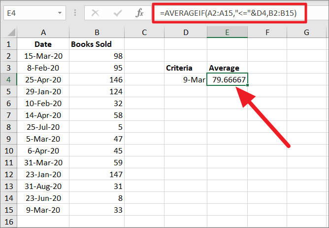
You can achieve the same result with this formula:
=AVERAGEIF(A2:A15,"<="&D4,B2:B15)Here, we are conjoining the logical operator with the cell reference using the ‘&’ operator. The text, logical operators, and date must be enclosed in double quotation marks in the criteria argument.
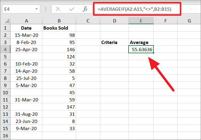
AVERAGE If Blank or Non-blank Cells
By default, the AVERAGEIF function ignores blank cells, but sometimes, we need to calculate the average value that corresponds either to blank or non-blank cells. In the criteria, we can use equal to in double quotes "" to find blank cells or <> to find non-empty cells.
Average If Blank
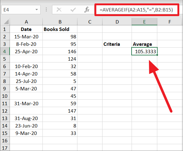
If you want to include truly blank cells (contain nothing) in the average, you can use "="in the criteria argument.
In the below data set, we wish to calculate the average for numbers that has absolutely nothing in the corresponding cells. To do that, we can use the below formula:
=AVERAGEIF(A2:A15,"=",B2:B15)The above formula calculates the average of the range B2:B15, only if the cell column A2:A15 in the same row is truly empty.
As you can see, cells A5, A10, and A12 are blanks, so the formula takes 124, 45, and 147 from column B corresponding to those cells and evaluates the average for those values. The result is returned in cell E4.
However, sometimes cells may appear blank but not entirely blank instead they would contain space characters or empty strings returned by other functions.
To get the average of cells corresponding to visually looking blank cells, enter the empty double quotes as criteria in below formula:
=AVERAGEIF(A2:A15,"",B2:B15)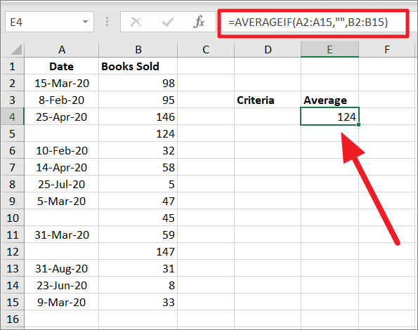
Average If Not Blank
In case you want to find the average of non-blanks, use the ‘not equal to’ operator (<>) in the criteria argument. To get the average value of non-empty cells, type the below formula:
=AVERAGEIF(A2:A15,"<>",B2:B15)Here, the formula evaluates the average of the numbers in B2:B15 if the corresponding cell in the range A2:A15 is not empty.
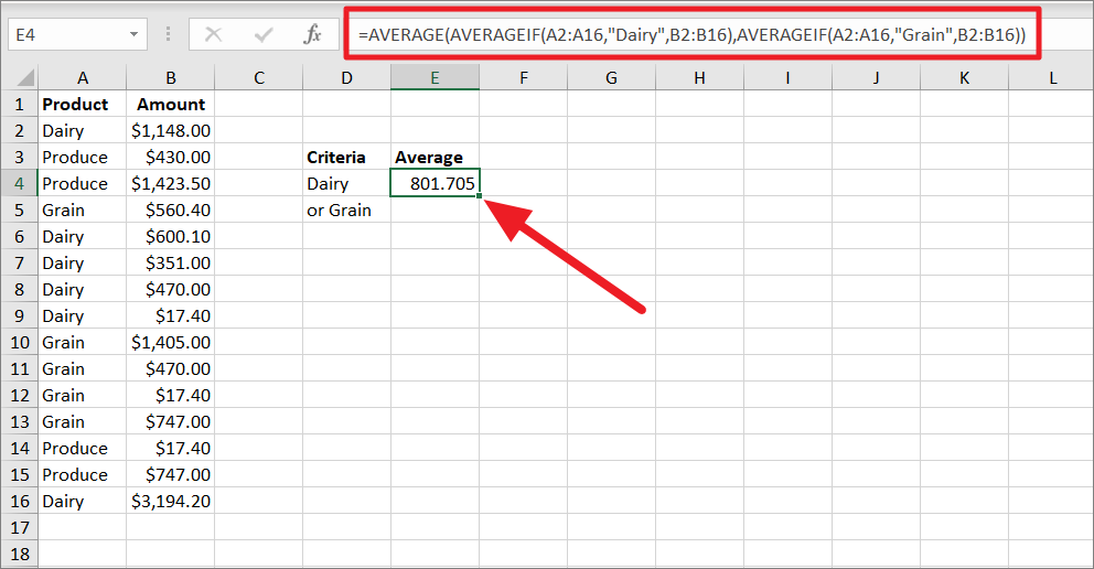
AVERAGEIF with OR logic (Multiple Criteria)
Usually, the AVERAGEIFS function is used to handle multiple Criteria but you can also use the AVERAGEIF function with AND or OR logic. You can add two or more AVERAGEIF functions inside the AVERAGE function to specify multiple conditions. If any of the given conditions are satisfied, the function finds an average of the corresponding values.
For example, we want to find the average of cells that satisfies either one of the criteria (‘Dairy’ or ‘Grain’) within the same range. This can be done by including two AVERAGEIF functions using OR logic.
To find an average of either Dairy or Grain, we can enter this formula:
=AVERAGE(AVERAGEIF(A2:A16,"Dairy",B2:B16),AVERAGEIF(A2:A16,"Grain",B2:B16))The above formula includes two AVERAGEIF functions – one for finding the average of ‘Dairy’ sales and another for finding the average of ‘Grain’. The first AVERAGEIF function averages the cells in B1:B16 when values in A1:A16 equal to Dairy and the second AVERAGEIF function average cells in B1:B16 when values in A1:A16 equal to Grain. Then, we average both results by nesting both AVERAGEIF functions within the AVERAGE function.
AVERAGEIF with AND logic (Multiple Criteria)
There may be times when you want to find the average of cells that satisfy all the given conditions. For that, you would have to use the AVERAGEIFS function which will combine AVERAGE and AND logic to get the average of values that meet all the conditions.
Using Wildcard Characters to Calculate Average based on Partial Match
Wildcards characters question mark (?), an asterisk (*), and tilde (~) can be used in criteria argument to find a value with a partial match.
The explanation for the three wildcard characters in Excel:
- Question mark (?) is used to match any single character or letter with the text string.
- Asterisk (*) is used to match any number of characters with the string.
- Tilde (~) is used to find an actual question mark or asterisk character.
Let us see how to wildcards to find the average based on a partial match:
Asterisk (*)
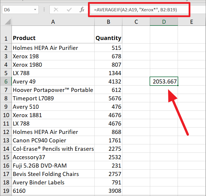
Suppose you have the below table and you want to find the average quantity of ‘Xerox’ products.
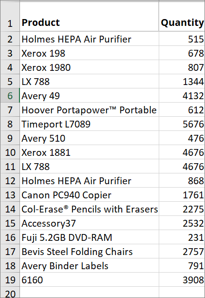
But the list contains different xerox products with different model numbers. If you simply use “Xerox” as criteria in the AVERAGEIF formula, you will end up with #DIV/0! error.
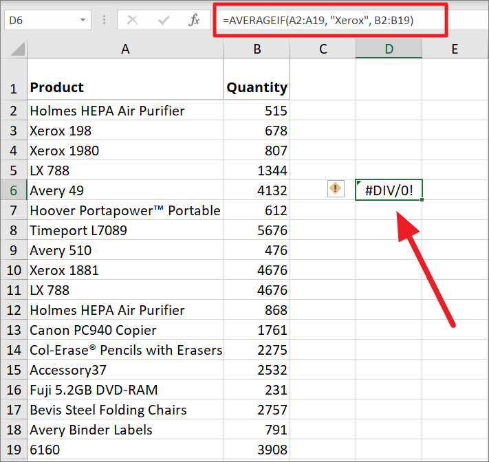
That is why you need to use an asterisk (*) to find the average for all Xerox products.
Example 1:
To average cells that partially match the given criteria, write the below formula:
=AVERAGEIF(A2:A19, "Xerox*", B2:B19)Here, we added an asterisk (*) character after the text ‘Xerox’ in the criteria, which means the formula looks for the word ‘Xerox’ followed by any number of characters in the range A2:A19. If the criteria is matched, it calculates the average with the corresponding values in the range B2:B19.
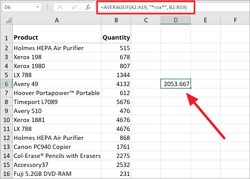
Example 2:
You can also use an asterisk (*) before and after the text to partially match the word that has other characters before and after it.
=AVERAGEIF(A2:A19, "*rox*", B2:B19)As you can see, the above formula produces the same result as the previous formula. Because the formula looks for product names with ‘rox’ in the middle which is preceded and followed by any other characters. Then it evaluates the average for the corresponding values.
Example 3:
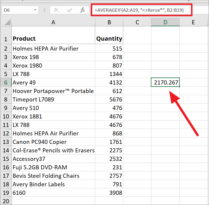
In case you need to find the average quantity of all items excluding any ‘Xerox’ product, write the below formula:
=AVERAGEIF(A2:A19, "<>Xerox*", B2:B19)This formula finds the average of all items except Xerox.
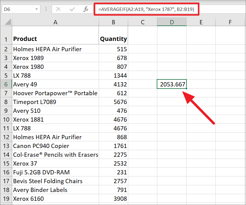
Question mark (?)
The question mark (?) wildcard can be used to match words with any single missing character.
Example 1:
For example, to calculate the average for cells that matches the given criteria with any two characters (in the wildcard place), use the below formula:
=AVERAGEIF(A2:A19, "Xerox 1?8?", B2:B19)In the above formula, we used two question marks (?) wildcards in the criteria (Xerox 1?8?) to represent any characters in their place. The formula matches the criteria with values in cells A3, A4, and A10. Then, calculates the average for the corresponding values in the range B2:B19.
Example 2:
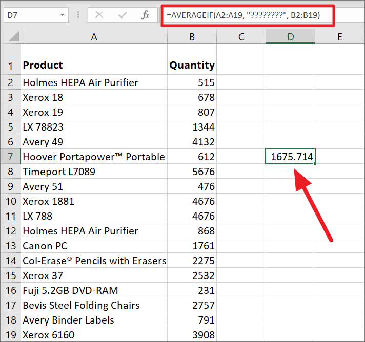
To calculates the average for cells that contain exactly 8 characters in the range A2:A19:
=AVERAGEIF(A2:A19, "????????", B2:B19)The above formula looks for values that contain any 8 characters in the range A2:A19 and if found, it calculates the average of corresponding values in the range B2:B19.
Here’s the list of wildcards criteria examples:
| Criterion Example | Explanation |
|---|---|
| “Excel” | The same as Excel |
| “Excel*” | Excel with suffix (of any number of characters) |
| “*Excel” | Excel with prefix (of any number of characters) |
| “E*l” | ‘E’ as prefix and ‘l’ as a suffix with any number of characters in between |
| “Exce?” | ‘Exce’ as a prefix with any one character suffix |
| “?xcel” | Any one character prefix with ‘xcel’ as suffix |
| “Exc?l” | ‘Exc’ as prefix, any one character in between, and ‘l’ as suffix. |
| “Excel~*” | Excel followed by a ‘asterisk (*)’ character |
| “Excel~?” | Excel followed by a ‘question mark (?)’ character |
Use the AVERAGEIFS function to Handle Multiple Criteria
The AVERAGEIFS function is a sibling (plural counterpart to the AVERAGEIF function in Excel. Unlike the AVERAGEIF function, AVERAGEIFS (plural counter) can handle multiple conditions at the same time. It means that all the provided conditions must be met to average the cells. The function was introduced in Excel 2007 and it is available in all later Excel versions.
Syntax of AVERAGEIFS function
=AVERAGEIFS(average_range, criteria_range1, criteria1, [criteria_range2, criteria2], …)The AVERAGEIFS function has the below arguments:
- average_range (required) – The range of cells that contain the values you want to average if multiple conditions are met.
- criteria_range1 (required) – This is the first range against which the first criteria is evaluated.
- criteria1 (required) – It is the first criteria that will be tested against the criteria_range1 to determine which cells will be averaged.
- criteria2, … – This is the second range against which the second criteria is tested. The criteria can be given in the form of a number, logical expression, text value, or cell reference.
- criteria_range2, … – This is the second criteria that will be tested against the criteria_range2 to determine which cells will be averaged.
Average Based on Multiple Criteria on a Single Column
You can apply the AVERAGEIFS function on a single column to calculate the average.
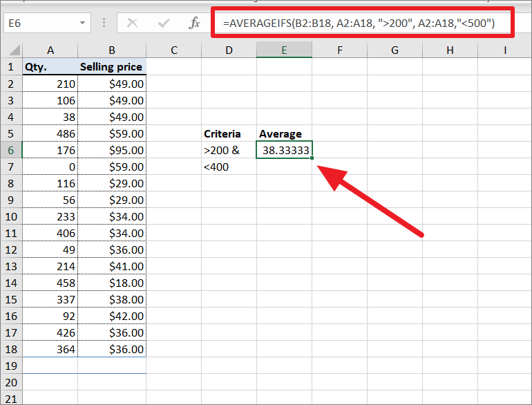
Let’s assume you have the below table where we have the number of items in the stock and their selling price.
Now, we want to find the average price of items that are greater than 200 and less than 400 in quantity. To do that, we can use the below formula:
=AVERAGEIFS(B2:B18, A2:A18, ">200", A2:A18,"<500")Here, we specified the start and endpoints of the range (Quantity) that we want to find the average for. With both criteria, the formula checks each cell in column A whether it is greater than 200 and less than 400. If both conditions are true, it takes out the corresponding selling price from column B. Then, it will calculate the average for all those numbers that satisfy both criteria.
Average Based on Multiple Criteria (Text and Date Criteria)
The AVERAGEIFS (Plural counterpart) is very similar to the normal AVERAGEIF, except you will need to provide more than one condition and criteria range in the formula. But all the conditions or criteria must be satisfied (AND logic) to average the cells.
Example 1:
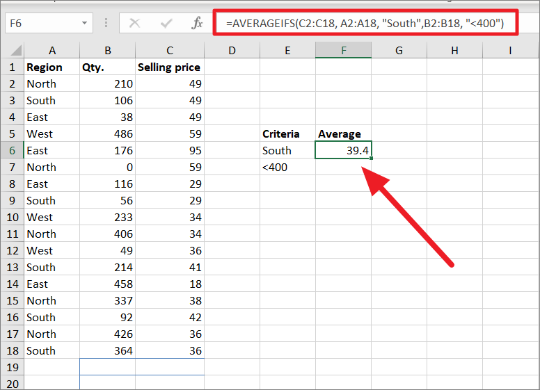
Suppose you have the below table and you want to find the average of sales in the North that are less than 400 in number, you can use the below formula:
=AVERAGEIFS(C2:C18, A2:A18,"South",B2:B18,"<400")Here, the formula checks each row if the value ‘South’ is in column A and the value in column B is less than 400. If both conditions are met, it takes out the corresponding numbers in column C and calculates the average for them.
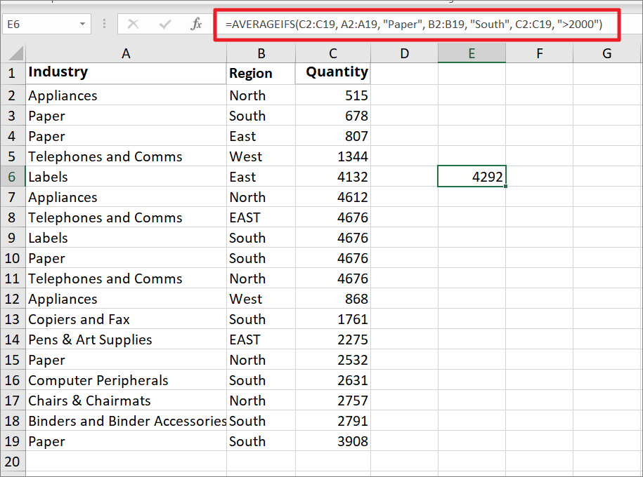
Example 2:
Let’s assume we wish to know the average number of paper products shipped to the Southern region that are greater than 2000. We can do that with the following formula:
=AVERAGEIFS(C2:C19, A2:A19, "Paper", B2:B19, "South", C2:C19, ">2000")Here is the list of items in column A, a region in column B, and the number of products shipped in column C. The above formula includes three criteria – two texts and one combination of logical operator and number. All three criteria must be satisfied to return the result.
Average Cells based on Multiple Criteria (Date criteria)
Just like with the AVERAGEIF function, you can also use Date as one of the multiple criteria in the AVERAGEIFS function.
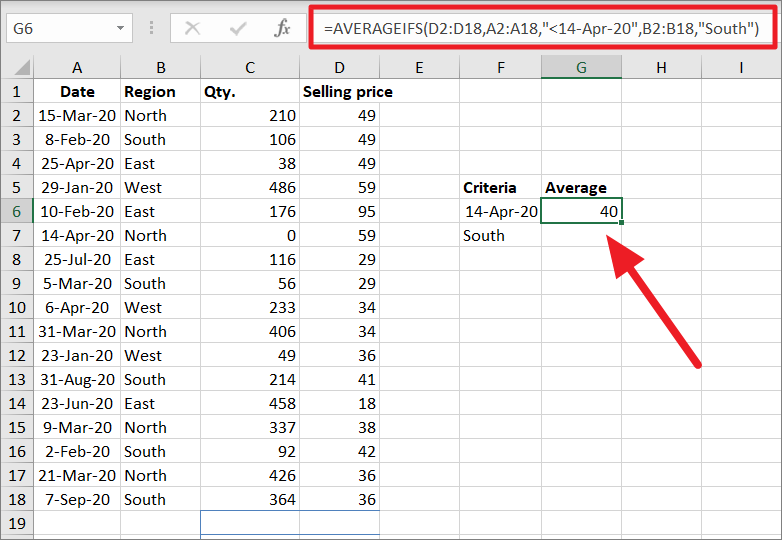
In the below example, let us find the average price for products sold before April 14 in the South region. To do that, we can use the below formula with multiple criteria, one for date and another for region:
=AVERAGEIFS(D2:D18,A2:A18,"<14-Apr-20",B2:B18,"South")In the formula, average_range is specified as column D, criteria_range1 is column A, criteria1 is ‘<14-Apr-20’, criteria_range2 is column B, and criteria2 is ‘South’.
The formula checks if the region ‘South’ and any date that is prior to ’14-Apr-20′ is in the same row. And if those conditions are satisfied, it calculates the average with the corresponding values in column D.
Calculate Average using AVERAGEIFS with OR logic
As we have seen above, the Excel AVERAGEIFS function uses AND logic to find the average of cells that meet all of the criteria and AVERAGEIF handles only one condition, but you can also employ the AVERAGEIFS function average cells by multiple criteria with OR logic. It can be done by adding more than one AVERAGEIFS function in the formula.
Example 1:
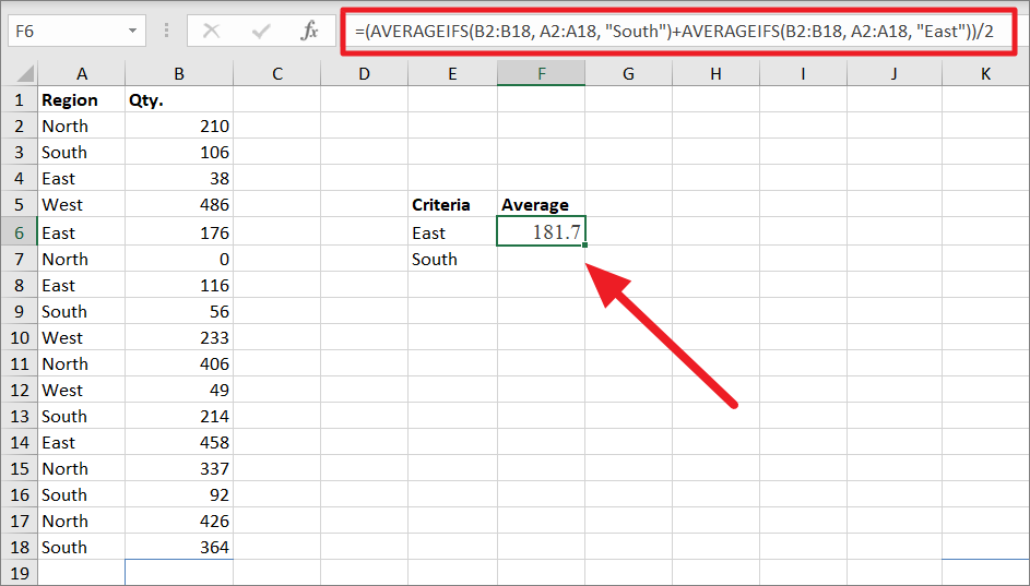
To find the average number of items sold in the south or north, try the below formula:
=(AVERAGEIFS(B2:B18, A2:A18, "South")+AVERAGEIFS(B2:B18, A2:A18, "East"))/2In the above formula, the first AVERAGEIFS function calculates the average quantity in column B if the corresponding row in column A is equal to ‘South’. Similarly, the second AVERAGEIFS function calculates the average quantity in column B if the corresponding row in column A is equal to ‘East’. Then, the result of both averages is summed up and divided by 2 to get the average number of items sold in the south or north.
Example 2:
In case you have to add more than two criteria to the formula, you can enclose the criteria inside an array to avoid rewriting the whole formula repeatedly.
Try this formula to get the same result as the previous formula:
=AVERAGE(AVERAGEIFS(B2:B18, A2:A18, {"South","East"}))In the previous example, we had to manually tell Excel to add two different AVERAGEIFS together and divide the result by 2. Here, Excel automatically finds the average for East and South by enclosing criteria inside an array as shown below. Also, this formula can significantly reduce the size of the formula no matter how many criteria you have to include.
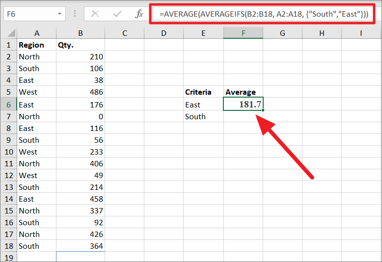
When Excel evaluates the formula, it automatically assumes we want to calculate the AVERAGEIFS for each criterion in the given array.
=AVERAGE(AVERAGEIFS(B2:B18, A2:A18,{166.4,197}))
Then, the outer AVERAGE function will add up the results and give you the final result.
=AVERAGE(166.4,197)
=181.7
Using Wildcards in Multiple Criteria of AVERAGEIFS function
You can also use wildcards question mark (?), an asterisk (*), and tilde (~) in multiple criteria of AVERAGEIFS function to average values.
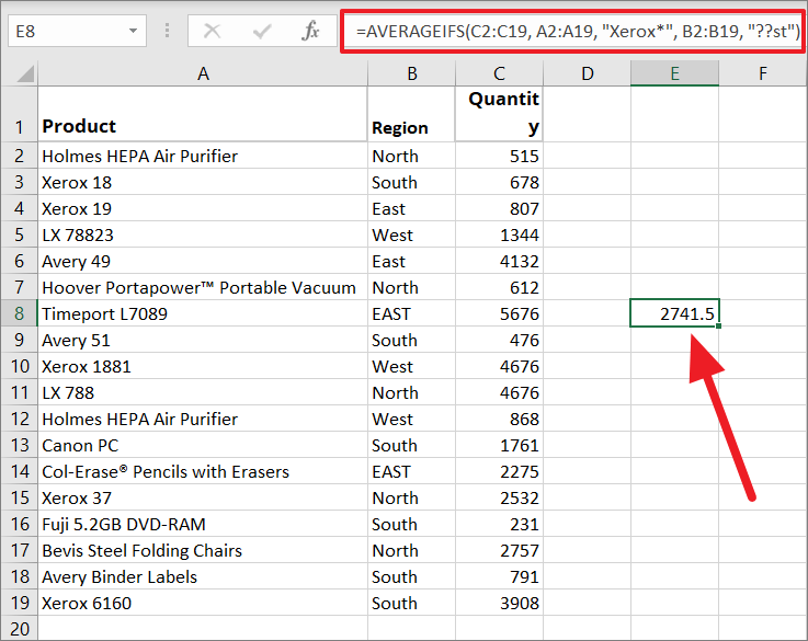
For example, we want to find the average of all Xerox products sold in East or West:
=AVERAGEIFS(C2:C19, A2:A19, "Xerox*", B2:B19, "??st")In the above formula, the criteria Xerox* matches with all the Xerox products in column A and ??st matches with South or East corresponding to any of those Xerox products. When both conditions are satisfied, it calculates the average quantity from column C.
Flexible AVERAGEIF Formula in Excel
If you have a large data set and you want to find the average for different items in that list, you can create flexible AVERAGEIF formula with a drop-down list to input criteria.
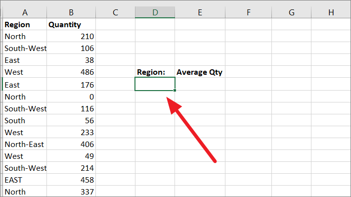
Suppose, you have the below dataset with the number of sales in differnt regions and you want to find the average quantity for different regions.
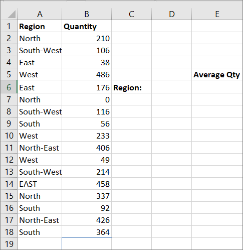
To start with, let’s extract the unique values we want to include in the drop-down from the ‘Region’ column.
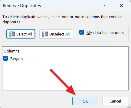
To do that, copy the column of values A2:A18 to a differnt location. Then, select that range of cells and go to the ‘Data’ tab on the top of the screen.
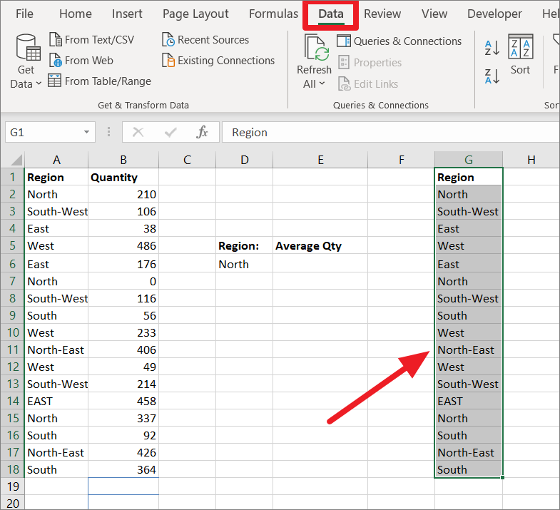
Under the Data tab, click the ‘Remove Duplicate’ button in the Data Tools group.
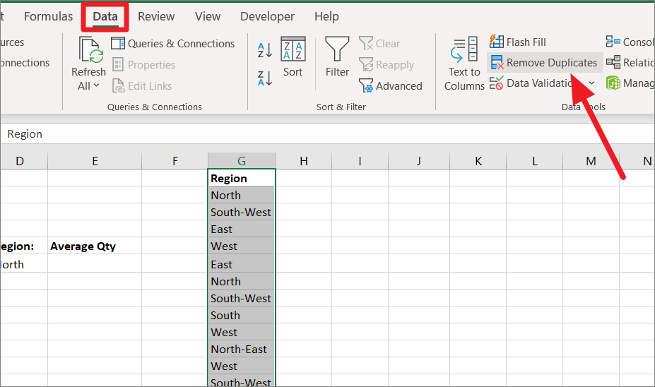
In the Remove Duplicates dialog box, make sure the column name (Region) is checked and click ‘OK’.
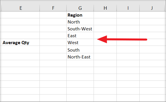
Now, we got the list of unique values from the Region column.
You can also type the unique values manually in a separate column.
Next, we need to create a drop-down list using the unique values we got. To do that, first, select a cell where you want to add the drop-down list.
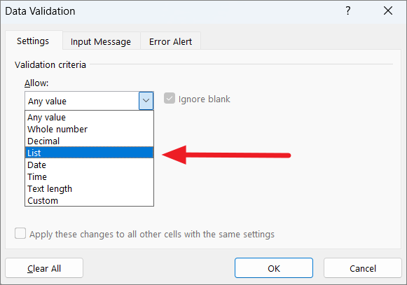
Then, go to the ‘Data’ tab and click the ‘Data Validation’ button from the ribbon.
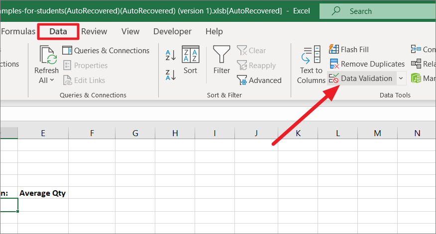
In the Data validation dialog window, choose ‘List’ from the Allow drop-down under Validation Criteria.
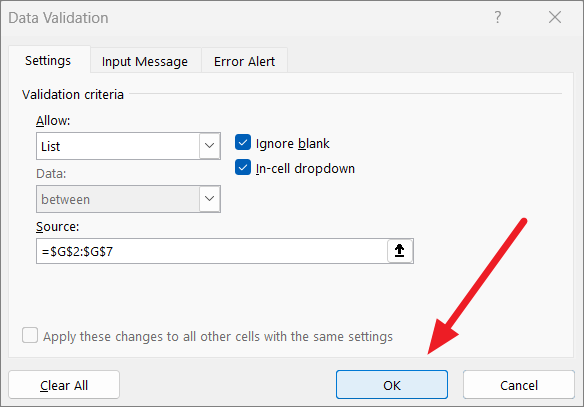
Next, click on the ‘Source’ field and select the range of cells that you want in your drop-down list.
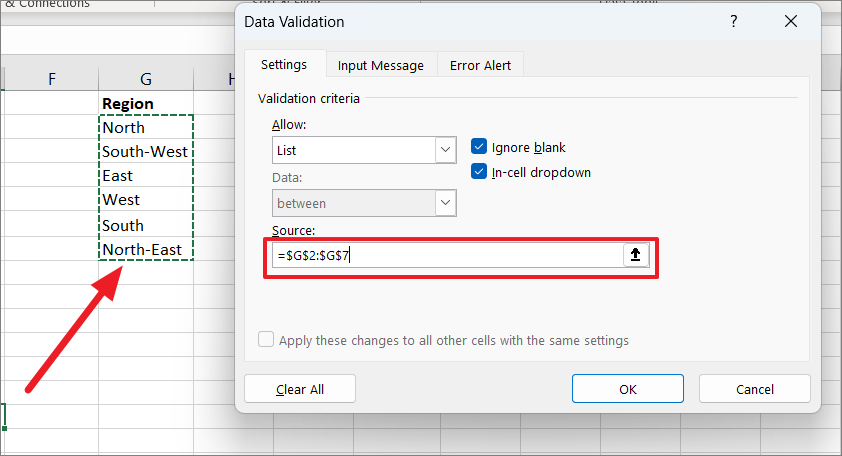
Then, click ‘OK’.
Now, you got your drop-down list with all the regions from column A.
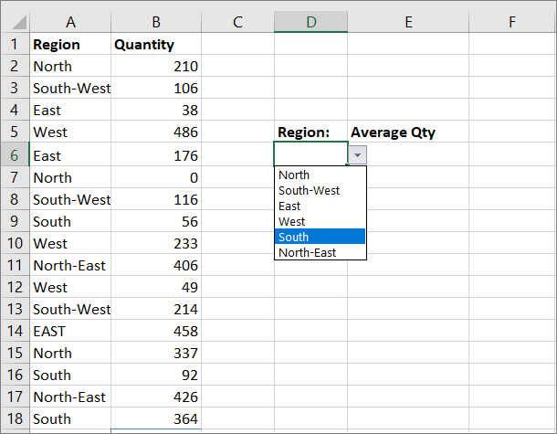
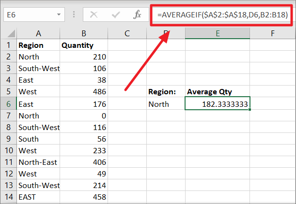
After that, we need to create a formula that takes criteria from the drop-down list in cell D6.
To calculate the average sales quantity for the select the region, enter the below formula:
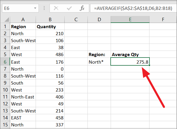
=AVERAGEIF($A$2:$A$18,D6,B2:B18)Here, we made the range argument absolute by adding dollar symbols ($A$2:$A$18), so it doesn’t change when the criterion is adjusted. The formula calculates the average quantity in the range B2:B18 if the selected criteria (Region) in D6 are met.
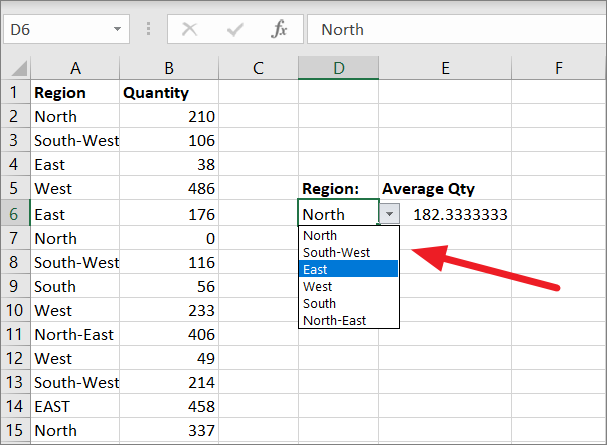
You can then use the drop-down list to change the criteria (Region) and the average value will automatically update for the selected criterion. The below screenshot shows the average for the North region.
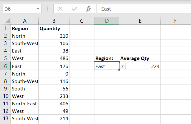
If we change the criterion to East, the average will automatically change according to that.
If we want to get the average of all of the northern regions including ‘North’ and ‘North-East’, we can add the asterisk (*) wildcard followed by ‘North’ in the cell D6 as shown below
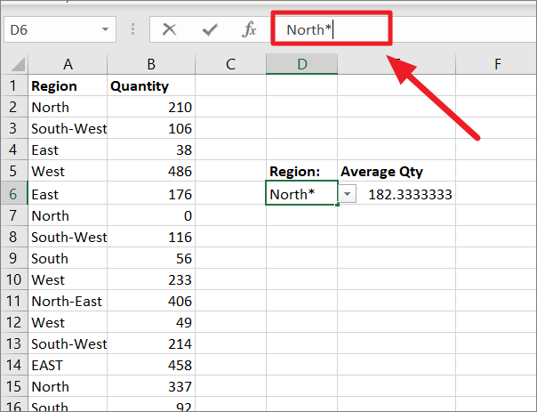
The AVERAGEIF will show the average for both North and North-East regions.
Why is the AVERAGEIF formula Not Working?
There are several reasons why your Excel AVERAGEIF function is not working. Here’s a list of reasons you can watch out for:
AVERAGEIF Supports Only One Condition
Unlike the AVERAGEIFS (Plural), the AVERAGEIF function only supports one criterion. If you enter multiple criteria, you will see the ‘You’ve entered too many arguments for this function warning’. Click ‘OK’ and check your formula.
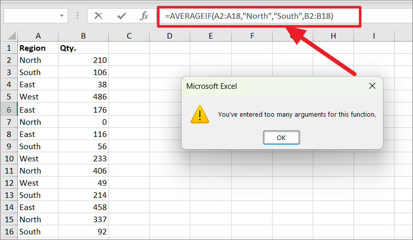
If you want to calculate the average with multiple criteria, you can either use an AVERAGEIF with multiple OR criteria or the AVERAGEIFS function (AND criteria).
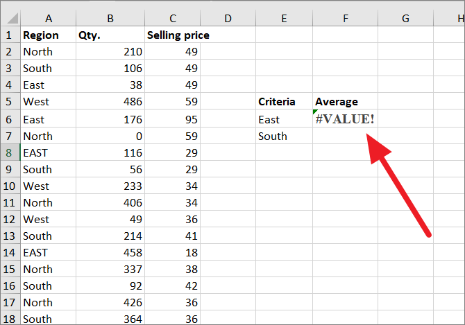
Range/Criteria_range and Average_range Should be the Same Size
In the AVERAGEIF formula, range/criteria_range and average_range should always be the same size, otherwise, you would get a #VALUE error.
As you can see below, the number of rows for the range and average_range arguments is not of the same size, hence the value error as the result (F6).
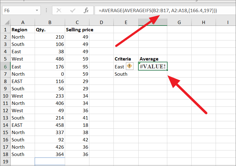
So, make sure to provide the same number of rows and columns (same-size range) for the range and average_range arguments in the formula.
Also, you cannot use arrays in range and average_range arguments in the AVERAGEIF function.
AVERAGEIF from Another Workbook is Not Working
You can use AVERAGEIF function to calculate the average for values from another worksheet or workbook by referring to the worksheet in the argument. But this will only work if the worksheet or workbook you are referring to is currently open.
For example, the below formula finds average for values from another workbook:
=AVERAGEIF([Book1.xlsx]Sheet1!A2:A18, "East", [Book1.xlsx]Sheet1!B2:B18)Here, [Book1.xlsx]Sheet1! refers to Sheet 1 in another workbook called Book1.xlsx.
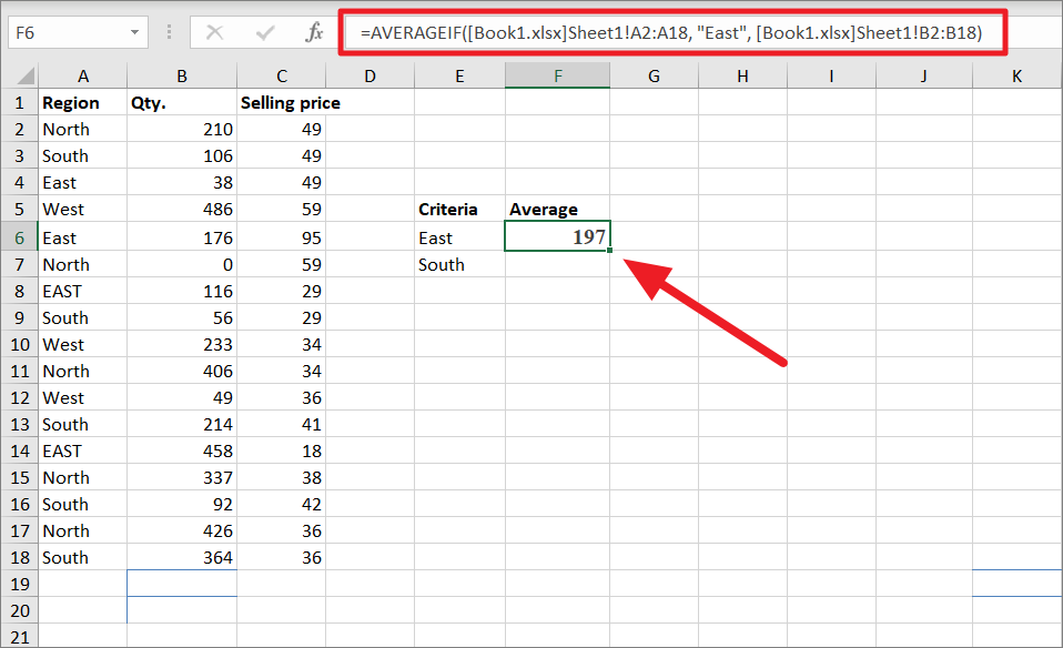
It will only work if the sheet the formula refers to is still open. The referenced range turns into arrays that are not supported by the range and sum_range arguments, hence the AVERAGEIF results in #VALUE! Error.
AVERAGEIF Criteria Argument
As you know, the AVERAGEIF function allows different types of values for criteria argument text, numbers, dates, cell references, logical operators, wildcard characters, and other formulas
If the criteria argument contains a text value, wildcard character, or logical operator followed by text, number, or date, enclose the whole criteria in double quotation marks.
Here’s a list of examples:
=AVERAGEIF(A2:A18, "East?", B2:B18)=AVERAGEIF(A2:A18, "<>East", B2:B18)=AVERAGEIF(A2:A18, "<=9/10/2020", B2:B18)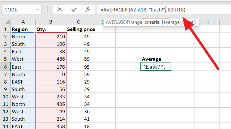
Also, if a cell reference or another function follows the comparison operator, enclose the logical operator in double quotation marks. Then, add an ampersand (&) symbol to concatenate (join) the logical operator and a reference or function as shown in the below examples:
=AVERAGEIF(A2:A18, ">"&G6, B2:B18)=AVERAGEIF(A2:A18, "<="&TODAY(), B2:B18)AVERAGEIF Function is Not Recognizing Particular Text
AVERAGEIF function is not case sensitive which means it evaluates uppercase and lowercase letters as the same characters. For instance, the text strings “WORKBOOK”, “workbook”, and “Workbook” will be treated as equal. It will calculate the average for all text no matter uppercase or lowercase.
Things to Remember About the AVERAGEIF Function
- If the cell(s) in the specified range contains Boolean values (TRUE or FALSE), they are ignored.
- Empty cells in the range and average_range are ignored by the AVERAGEIF.
- If the given criteria is empty, the AVERAGEIF handles it as a 0 value.
- If the average_range is blank or contains a text value, the AVERAGEIF formula returns the #DIV0! error as the result.
- If no cells in the range meet the criteria, the formula returns the #DIV/0! error.
- If values the in average_range cannot be translated into numbers, the formula returns the #DIV0!.
- If the range and average_range are not of the same size or if the text criteria exceed the length more than 255 characters, the formula returns the #VALUE! error.
- If a number or date is joined with a logical operator in the criteria argument, the whole argument must be enclosed in double quotation marks. e.g. “>5/10/2022”.
- As we mentioned before, you can use wildcard characters, question marks (?), and asterisk (*) characters in the formula as criteria argument.
That’s it.


