
The sum is the addition of values and the product is the multiplication of values. Hence, the SUMPRODUCT function is used to multiply cell values, and then sum their resulting products. It is one of the most useful and advanced mathematical functions in Excel. It is used to multiply the numbers in corresponding arrays or ranges and return the sum of those product results.
SUMPRODUCT is a highly versatile function and it can be used for many purposes like counting cells, summing values based on multiple criteria, looking up values, comparing data between two ranges, and more. It is also often used to calculate a weighted average. Besides addition and subtraction, it can also be modified to perform subtraction and division as well.
In this post, we will discuss what is SUMPRODUCT function, and its basic and advanced uses in Excel with examples.
What is SUMPRODUCT function?
The SUMPRODUCT function is designed to multiply corresponding arrays or rangers and then aggregate results.
Syntax
=SUMPRODUCT(array1, [array2], [array3],...)Arguments:
- array1 (required) – This is the first array or range of cells whose values you want to multiply and then add.
- [array2], [array3],… (optional) – This is the second (and third) array or range of cells whose values you want to multiply and then add. The function takes up 30 arrays in old Excel versions but in the modern versions, it can accept up to 255 arrays.
The array or ranges of cells must have the same number of columns or rows, otherwise, you will get an #VALUE! error. If there are any non-numeric arrays values in the arrays, they will be treated as zero.
Basic Use Of SUMPRODUCT Function
To know the SUMPRODUCT function better, first, let us see how the function works with some basic examples.
Example 1:
For example, let us assume you have the below table that contains a list of products, their quantity & price.
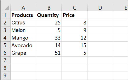
Now, you want to find the total cost of all products. To do that, you can use the below formula:
=SUMPRODUCT(B2:B6,C2:C6)The above formula multiplies each from B2:B6 with the corresponding cells C2:C6 and sums up the multiplication results.
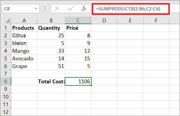
This is what the SUMPRODUCT function’s operation looks like inside the formula:
=(B2*C2)+(B3*C3)+(B4*C4)+(B5*C5)+(B6*C6)
=(25*8)+(5*9)+(33*12)+(14*15)+(51*5)
=200+45+396+210+255=1106
Example 2:
In the above formula, both array 1 and array 2 have single columns. So it multiplies two single columns of numbers and summed up their results. But if your arrays consist of multiple columns (e.g. B2:C6), you can write a formula like this:
=SUMPRODUCT(B2:C6,D2:E6)The formula multiplies each value of A2:B6 to the corresponding value of B2:C6 and then aggregates all the product values:
=(B2*D2)+(B3*D3)+(B4*D4)+(B5*D5)+(B6*D6)+(C2*E2)+(C3*E3)+(C4*E4)+(C5*E5)+(C6*E6)
=(25*8)+(5*9)+(33*12)+(14*15)+(51*5)+(17*9)+(7*7)+(53*15)+(24*28)+(82*6)
=200+45+396+210+255+153+49+795+672+492
=3267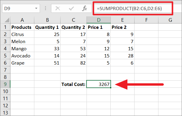
Example 3:
No matter how many arrays you specify in the SUMPRODUCT function, all of them should be the same size, otherwise, you would get a #VALUE error. In the below formula, the arrays B2:B6 and C2:C7 are mismatched, hence, the #VALUE error.
=SUMPRODUCT(B2:B6,C2:C7)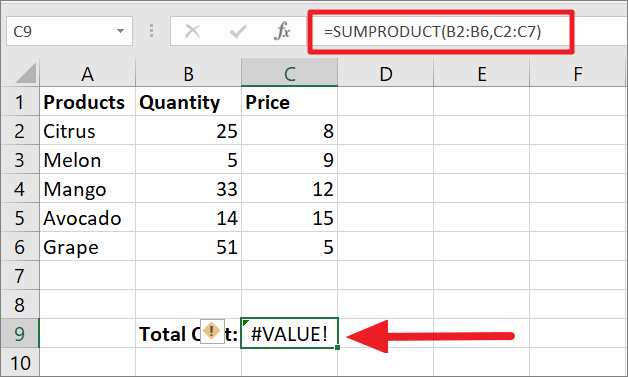
Perform Other Arithmetic Operations using SUMPRODUCT
The SUMPRODUCT can also be used to perform other arithmetic operations such as division, addition, or subtraction of arrays. To do this, all you have to do is separate each array with the proper mathematical operators (+,-,/) instead of default comma (,). Then, the function will perform the user-specified mathematical operations and sum up the results. By using mathematical operators, you can also customize the operations between arrays. Let us see how to do this with some examples:
SUMPRODUCT for Addition:
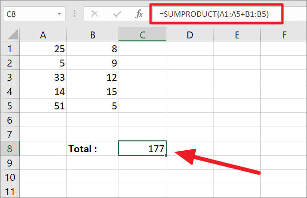
To add two arrays of numbers (instead of multiplying) them and then add up the results, you need to use the below formula:
=SUMPRODUCT(A1:A5+B2:B5)Here, the function adds each value with the corresponding cell values and adds ups the result.
SUMPRODUCT for Subtraction:
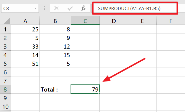
In case you want to perform subtraction operations instead of multiplication, write a formula similar to this:
=SUMPRODUCT(A1:A5-B1:B5)Here, the formula subtracts each value from A1:A5 from the corresponding B1:B5 and sums up the resulting values.
SUMPRODUCT for Division:
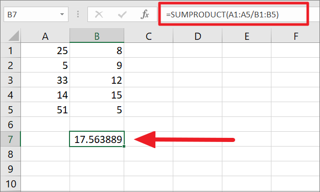
If you want to use SUMPRODUCT for division, use the below formula:
=SUMPRODUCT(A1:A5/B1:B5)The above formula divides the value in A1 by the value in B1, value in A2 by B2, and then A3 by B3, and finally adds up all the results to provide the result: 17.563
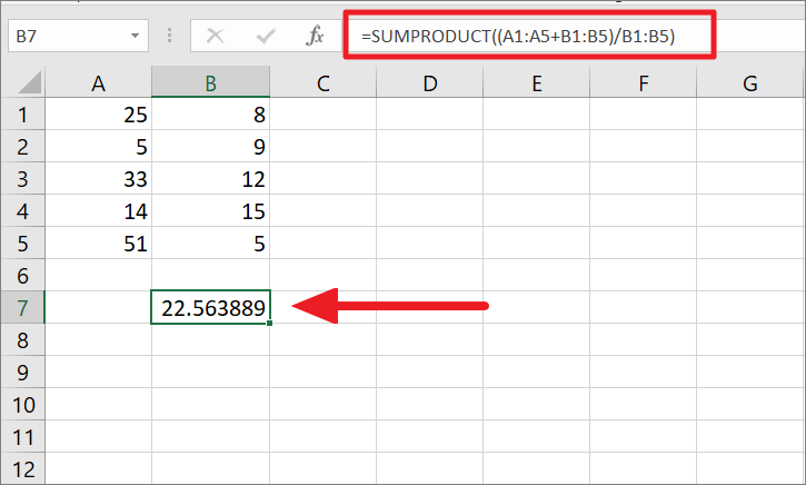
With SUMPRODCUT Function, you can also customize the arithmetic operations between the array elements (arguments) by using different operators.
=SUMPRODUCT((A1:A5+B1:B5)/B1:B5)Here, the formula adds the ranges A1:A5 and B1:B5 first because it is enclosed in parentheses, and resulting values are divided by B1:B5, which outputs the result: 22.56.
SUMPRODUCT with One Criteria
Sumproduct can be used to sum or count the values that meet a particular condition or criteria like SUMIF and COUNTIF but with more flexibility. First, let us see how you can do that with a single criterion.
Syntax
=SUMPRODUCT(--(criteria_range=criteria),sum_range)Where
- sum_range – The range or array where you want to sum the values if the condition is met.
- criteria – This is the condition that needs to be met to sum the values.
- criteria_range – The array or range where the condition is checked.
To check a condition, we have to use a logical operation that only results in Boolean values (TRUE or FALSE). But multiplying TRUE or FALSE with the sum_range will only result in 0s. So, to convert those boolean values into usable 1s (TRUE) and 0s (FALSE), we need to enclose the condition in brackets and add a double negation operator (–) before that.
Example 1:
For instance, you have a data set as shown below where you want to find out the total sales of ‘Oranges’.
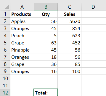
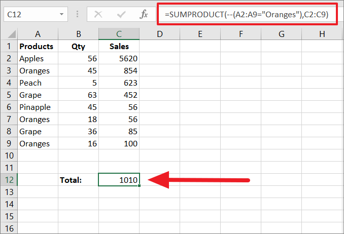
To sum the total sales of Oranges, use the below formula:
=SUMPRODUCT(--(A2:A9="Oranges"),C2:C9)In the above formula, A2:A9="Oranges" returns an array of logical values: {FALSE, TRUE, FALSE, FALSE, FALSE, TRUE, FALSE, TRUE}. The formula only returns TRUE for the cells that contain the value “Oranges” in the range A2:A9 and for the cells that contain other values, it returns FALSE. And the double negation (double minuses) converts these values into an array of 1s and 0s: {0, 1, 0, 0, 0, 1, 0, 1}.
This is what the formula will look like after that:
=SUMPRODUCT({0, 1, 0, 0, 0, 1, 0, 1}, {5620, 854, 623, 452, 56, 56, 85, 100})
=(0, 1, 0, 0, 0, 1, 0, 1) x (5620, 854, 623, 452, 56, 56, 85, 100)
=854+56+100
=1010
Then, SUMPRODUCT then multiples each value in array1 with the corresponding value in array2, and then adds up the resulting array: 1010.
Example 2:
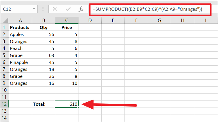
You can also use the SUMPRODUCT formula to find the sum product of values that meets a specific condition. For example, in the below example we want to multiplication Sumproduct for two arrays but only for the product named ‘Oranges’.
To do that, use the below formula:
=SUMPRODUCT((B2:B9*C2:C9)*(A2:A9="Oranges"))Here, the formula A2:A9="Oranges" searches for the product names ‘Oranges’ in the range A2:A9 and returns the array – {FALSE, TRUE, FALSE, FALSE, FALSE, TRUE, FALSE, TRUE}. Then, the formula multiplies the two arrays B2:B9 and C2:C9 and returns another array of results.
There is no need to use a double negation (–) before the condition argument because the multiplication operator between the two arguments also acts as a converter and forces the TRUE and FALSE values from (A2:A9=”Oranges”) to 1s and 0s. As a result, only the values that have ‘Oranges’ in the range will have 1 as the results. So, the formula will load into like this: =SUMPRODUCT({280, 360, 30, 252, 225, 90, 288, 160}*{0, 1, 0, 0, 0, 1, 0, 1}). Hence, we get ‘610’ as the output.
SUMPRODUCT with Multiple Criteria
SUMPRODUCT is a good alternative to both COUNTIFS and SUMIFS to count and sum values based on multiple conditions. Unlike COUNTIFS and SUMIFS, it can work with both AND and OR logic formulas.
Sum Cells Based on Multiple Criteria with AND Logic
For AND logic formula, all conditions or criteria must be met on a row to sum the corresponding values in the specified array.
Syntax
=SUMPRODUCT(--(criteria_range1=criteria1),--(criteria_range2=criteria2), sum_range)To shorten the formula, you can also replace the comma between the array elements with the AND operator asterisk (*).
Example 1:
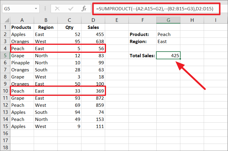
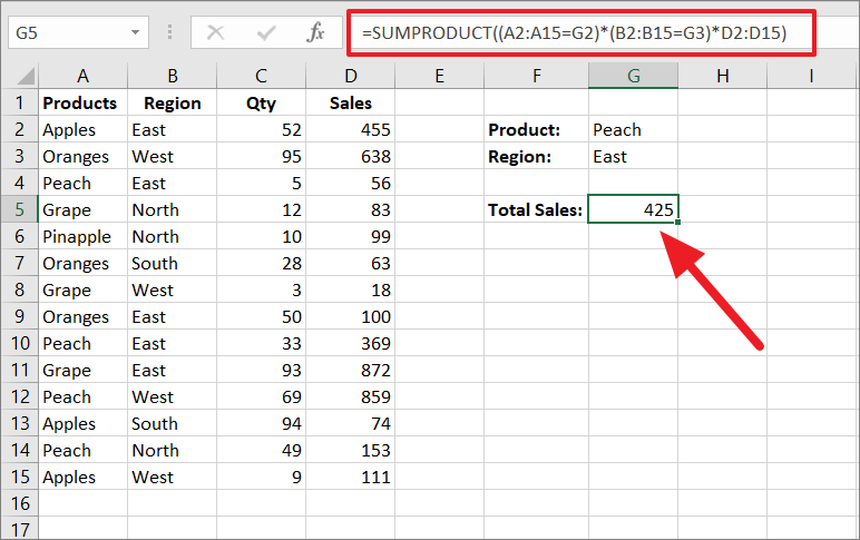
Suppose, we have the below dataset and we want to sum the total Sales values of ‘Peach’ fruit for the ‘East’ region.
To sum the total sales of ‘Peach’ fruit for the ‘East’ region, write the below formula:
=SUMPRODUCT(--(A2:A15="Peach"),--(B2:B15="East"),D2:D15)or
=SUMPRODUCT(--(A2:A15=G2),--(B2:B15=G3),D2:D15)Both of the above formulas give you the same result. But in the second formula, we referred to the cells that contain the criteria values to shorten the formula.
In the above formula, Peach and East are the two specified criteria.
A2:A15=G2checks the range A2:A15 for the value that is equal to the one entered in cell G2 (Peach) and return an array of true and false which is then converted by double negative (–) into this – {0, 0, 1, 0, 0, 0, 0, 0, 1, 0, 1, 0, 1, 0}. Here, 1 stands for Peach and 0 for other fruits.- Then
B2:B15=G3looks for the value entered in cell G3 (East) and returns this array of results – {1, 0, 1, 0, 0, 0, 0, 1, 1, 1, 0, 0, 0, 0}. Here, 1 stands for ‘East’ and 0 for any other region. - After that both resulting arrays are multiplied and outputted this array – {0, 0, 1, 0, 0, 0, 0, 0, 1, 0, 0, 0, 0, 0}. This means we only get ‘1’ if both conditions are met, 0 otherwise. As you can only row 3 and 10 have ‘1’ in the array of results because they are the only two rows that satisfy the specified criteria.
- Now, the final array of results is multiplied with the corresponding sales value in D2:D15. When multiplying 1 with a number gives the same number, multiplying 0 always gives us zero in return. As a result, only the sales value in rows 3 and 10 are added together to give us the result: 425.
Alternatively, you can perform the same above calculation using the below formula which is a bit shorter than the above formula:
=SUMPRODUCT((A2:A15=G2)*(B2:B15=G3)*D2:D15)In the above formula the Asterisk (*) is used to multiply the two conditions and the asterisk is also considered as the AND operator in SUMPRODUCT. If you add asterisk characters between arrays, you don’t need to add double negation (–) before the logical condition.
Example 2:
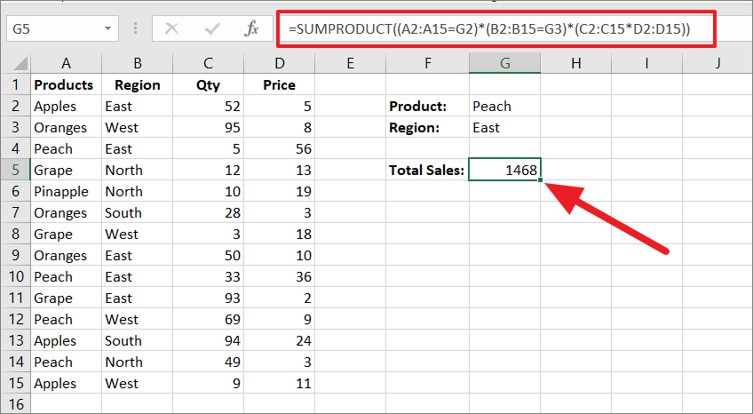
For example, find the total sales of Peach fruit in the East region by multiplying quantity and price and then sum up the results. To do that you can use the below formula
=SUMPRODUCT((A2:A15=G2)*(B2:B15=G3)*(C2:C15*D2:D15))This formula checks for the conditions (Peach and East) in columns A and Column B respectively. And if both values are found in the same row (if both conditions are met), the formula multiplies and adds the corresponding values in columns C and D.
Sum Cells Based on Multiple Criteria with OR Logic
Unlike COUNTIFS and SUMIFS, SUMPRODUCT allows you conditionally sum or count values with OR logic. For the OR logic formula, either of the criteria must be met on a row to sum the corresponding values in the specified array. To apply OR logic, you need to use plus symbol (+) in between the arrays instead of an asterisk.
The plus sign (+) works as an OR operator and returns TRUE if any of the given criteria in the formula evaluates to TRUE.
Syntax:
=SUMPRODUCT((criteria_range1=criteria1)+(criteria_range2=criteria2), sum_range)Example:
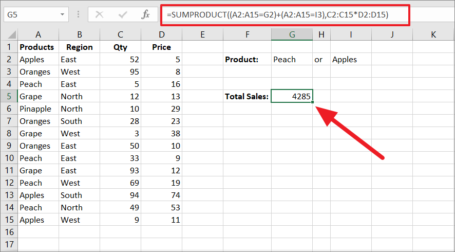
If you want to find the total sales of Peach and/or Apples regardless of the region, write a formula like the following:
=SUMPRODUCT((A2:A15=G2)+(A2:A15=I3),C2:C15*D2:D15)The above formula looks for the products ‘Apples’ (I2) and ‘Peach’ (G2) in column A and then multiplies corresponding values in column C (Qty) and D (Price) and adds up result if either of the condition is met. That means it will multiply columns C and D and add values for all Apples and Peach products regardless of the region.
Sum Cells Based on Multiple Criteria with AND as well as OR Logic
Sometimes, you may need to conditionally sum cells with both OR and AND logic at the same time, which you can easily do with the SUMPRODUCT function.
Example 1:
For instance, if you want to find the sum of Apples and Peach sales in the East region, this is what the combination of AND and OR logic will look like (syntax):
=Sum If ((Product="Apples") OR (Product="Peach")) AND (Region="East"))Now, apply the above logic into the actual formula by replacing ‘AND’ with (*) and OR with (+).
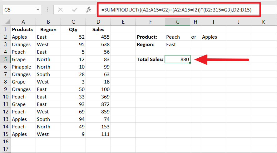
To sum ‘Peach’ and ‘Apples’ sales in the East region, use the below formula:
=SUMPRODUCT(((A2:A15=G2)+(A2:A15=I2))*(B2:B15=G3),D2:D15)Let’s breakdown the formula:
- In the formula, we have three conditions:
(A2:A15=G2)for ‘Peach’ in column A,(A2:A15=I2)for ‘Apples’ in column A, and (B2:B15=G3) for ‘East’ in column B. In order to sum the corresponding values in column D, either of the first two criteria must be satisfied (OR) and the third criteria must be satisfied (AND).
((A2:A15=G2)+(A2:A15=I2))part of the formula checks for either ‘Peach’ or ‘Apples’ item in Column A. If either of the items is found in the list A2:A15, it evaluates to TRUE (FALSE otherwise) which means ‘1’.(B2:B15=G3)checks for the value ‘East’ in column B and if it is found, it evaluates to TRUE, which is also converted to ‘1’.- When both array of results are multiplied from OR and AND logic, we will get this array – {1, 0, 1, 0, 0, 0, 0, 0, 1, 0, 0, 0, 0, 0}.
- Finally, the formula multiplies the final array of results with the column D values and then sums the result to – 880.
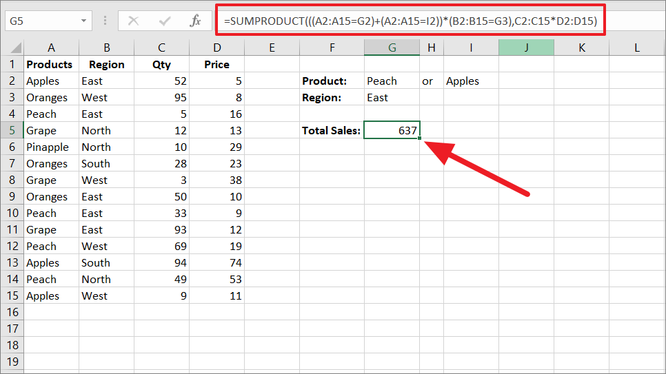
Example 2:
The above formula finds the sum of values based on multiple criteria with AND and OR logic. But if you want to find the Sum-Product of values, you need to use the below formula:
=SUMPRODUCT(((A2:A15=G2)+(A2:A15=I2))*(B2:B15=G3),C2:C15*D2:D15)This formula is nearly the same except we added another array into the formula. Now, if either ‘Apples’ or ‘Peach’ and the value ‘East’ is found in the same row, the corresponding values in columns C and D are multiplied and added up to give the output: 637.
Sum Cells using SUMPRODUCT and Exact Function
In case you need to look up a case-sensitive value and sum their corresponding values using the SUMPRODUCT function, you need to include the EXACT function inside the formula.
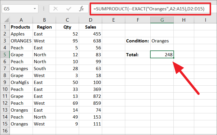
Let’s assume you have some case-sensitive values in a table and you want to sum the corresponding values, try the below formula:
=SUMPRODUCT(--EXACT("Oranges",A2:A15),D2:D15)The EXACT("Oranges",A2:A15) portion of the formula looks for the exact specified string (Oranges) with the same case characters in the range A2:A15. If a match is found, it returns TRUE or else FALSE. These true or false results are converted into numeric values by the double negative – {0, 0, 0, 0, 0, 1, 0, 0, 0, 0, 0, 1, 0, 1}. Then, the resulting array is multiplied with the sum array (D2:D15). And, the final product results are added up to give you the total sum – 248.
Count Cells using SUMPRDUCT function
We have seen how to conditionally sum cells in Excel, now, let us see how to count the cells that meet the criterion/criteria using the SUMPRODUCT function.
Syntax:
=SUMPRODUCT(--(array=condition))Count Cells with a Single Criteria
Let’s assume you have a list of fruits, their quantity, and price in columns A, B, and C respectively.
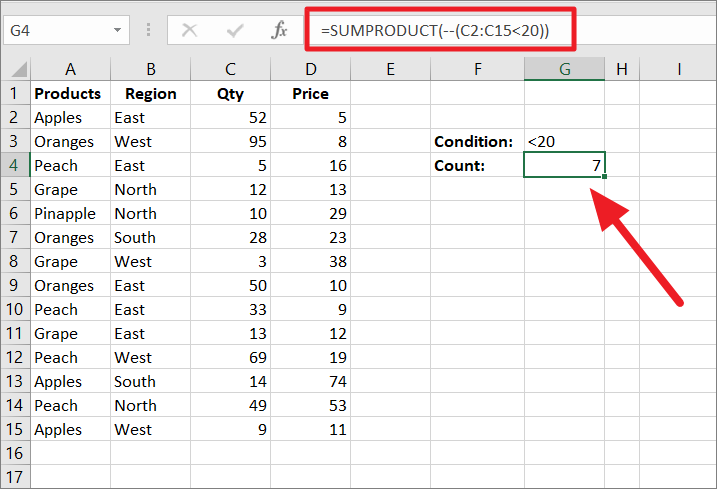
Now, we want to find out how many items that have less than 20 in quantity. To do that we can use any one of the below formulas:
=SUMPRODUCT(--(C2:C15<20))Where, C2:C15<20 condition checks whether each value in column C is less than 20 or not and returns this array of results –
{FALSE;FALSE;TRUE;TRUE;TRUE;FALSE;TRUE;FALSE;FALSE;TRUE;FALSE;TRUE;FALSE;TRUE}.
Then, the array of results is converted into 1s and 0s by the double negation: {0, 0, 1, 1, 1, 0, 1, 0, 0, 1, 0, 1, 0,1}. After that, the SUMPRODUCT sums up all the results to give us the count of cells – ‘7’.
Alternatively, you can also convert the boolean values into numeric values by multiplying the array of results by 1:
SUMPRODUCT((C2:C15<20)*1)Either way, both formulas will give you the same number of counts.
Count Cells Based on Multiple Criteria with AND Logic
If you have more than one condition and you want to count cells only when all those conditions are met, you can use the SUMPRODUCT formula with AND logic.
Example:
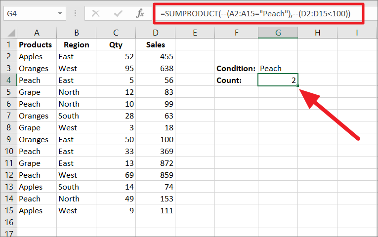
For example, if you want to count how many times the Peach sales were less than 100, you can add two criteria to the SUMPRODUCT formula – one to search the column A for ‘Peach’ item and another to check if the corresponding sales are less than 100:
=SUMPRODUCT(--(A2:A15="Peach"),--(D2:D15<100))or, if you want a short formula, you can try this instead:
=SUMPRODUCT((A2:A15=G3)*(D2:D15<100))A2:A15="Peach" or A2:A15=G3 checks for the ‘Peach’ item in the column A2:A15 and D2:D15<100 checks for sales amount that is less than 100. If both conditions are satisfied in the same row (row 4 and row 6), it counts those rows and returns the result.
Inside the formula, A2:A15="Peach" condition returns this array of converted results: {0, 0, 1, 0, 1, 0, 0, 0, 1, 0, 1, 0, 1, 0} and D2:D15<100 returns this array of converted results: {0, 0, 1, 1, 1, 1, 1, 0, 0, 0,0,1, 0, 0}. And when both are arrays are multiplied, you will get the count ‘2’.
Count Cells Based on Multiple Criteria with OR Logic
You can use the plus symbol (+) symbol in between the arrays to count cells with the OR logic.
Example:
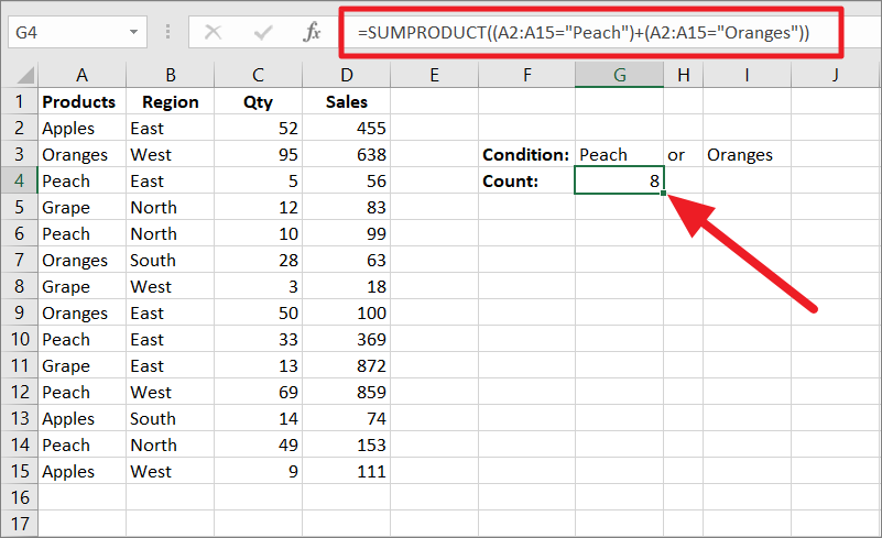
To find the count of Peach and Oranges sales regardless of the region, enter the below formula:
=SUMPRODUCT((A2:A15="Peach")+(A2:A15="Oranges"))In the above formula, the plus sign (+) between the arrays acts as an OR operator and returns the TRUE if any of the given two conditions are satisfied. If either of the ‘Peach’ or ‘Orange’ items is found in the list, the formula returns TRUE. The OR operator also acts as an convertor and produces this array of values: {0, 1, 1, 0, 1, 1, 0, 1, 1, 0, 1, 0, 1, 0}. Then, the resulting array is added to produce the output: 8.
Count Cells Based on Multiple Criteria with AND as well as OR Logic
Similarly, you can conditionally count cells using the SUMPRODUCT function with both OR and AND logic at the same time.
Example:
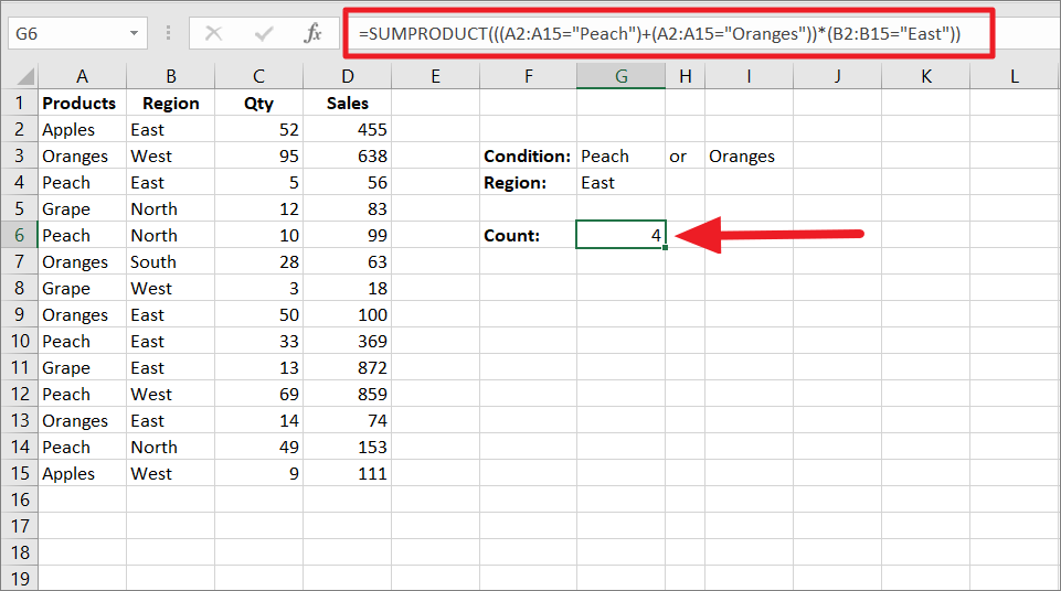
To find the number of Oranges and Peach sales in the East region, use the below formula:
=SUMPRODUCT(((A2:A15="Peach")+(A2:A15="Oranges"))*(B2:B15="East"))Here, (A2:A15="Peach")+(A2:A15="Oranges") portion of the formula checks for either ‘Peach’ or ‘Oranges’ item in A2:A15. If either of the items is found in column A, it evaluates to TRUE (FALSE otherwise) which is turned into ‘1’, otherwise ‘0’.
(B2:B15="East") searches for the value ‘East’ in column B and if it is found, it evaluates to TRUE, which is also turned into ‘1’. Then, both of the results from OR and AND logic are multiplied to produce – {0, 0, 1, 0, 0, 0, 0, 1, 1, 0, 0, 1, 0,0}. At last, the final array of results is summed up to – ‘4’.
Count Distinct Values using SUMPRODUCT and COUNTIF Formula
SUMPRODUCT formula is also helpful when you want to count distinct values from a list of values. The Distinct values are all the different values including the unique entries in a list. Distinct values are also considered unique values in some cases, so knowing how to find them is useful.
It doesn’t matter how many duplicates a value has, only one instance of that value is included in the count. For example, if the value ‘New York’ is repeated 5 times in a list, it is still counted as just ‘1’.
The easiest formula to count distinct values is a combination of SUMPRODUCT and COUNTIF.
Here’s the syntax to count unique and distinct values in a column:
=SUMPRODUCT(1/COUNTIF(data,data))Where data is the data range where you want to count values.
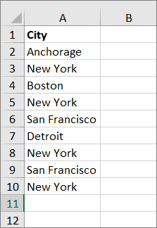
For example, we want to find the count of distinct values in the following list:
To do that use the following formula:
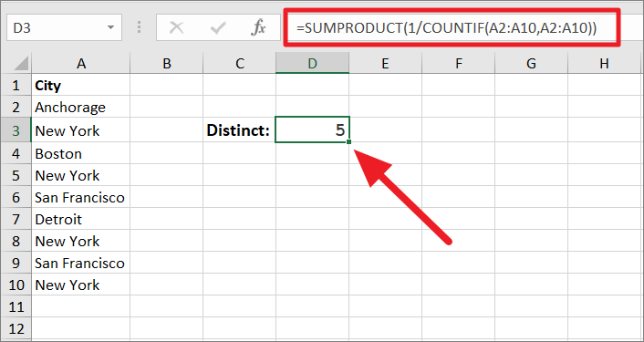
=SUMPRODUCT(1/COUNTIF(A2:A10,A2:A10))Let us break it down for you:
COUNTIF(A2:A10,A2:A10):The nested COUNTIF function counts the number of times each value appears in the cell range (A2:A10) and returns an array of numbers like this:{1;4;1;4;2;1;4;2;4}. i.e. The value that appears only once is 1, the value that appears 4 times is 4, etc.1/COUNTIF(A2:A10,A2:A10): After that, the resulting array of numbers from the COUNTIF formula is used as a divisor/divider for the division with1as their numerator. So 1 is divided by each value of COUNTIF’s array of results. As a result, you will get another array of result:{1;0.25;1;0.25;0.5;1;0.25;0.5;0.25}.
As you can see, the value that appears only once (unique) are 1, and values that appear multiple times will become fractions. For example, the value ‘San Francisco’ appears twice, so when 1 is divided by 2, you will get ‘0.5’.
Finally, the SUMPRODUCT function adds up all numbers in the array and returns the count of distinct values: ‘5’. The count includes all the different values that appear at least once in the list, excluding the duplicates.
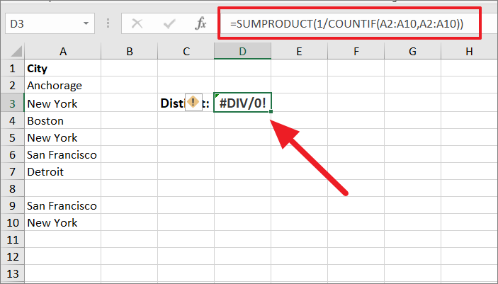
Count Distinct Values Ignoring/Including Blank Cells using SUMPRODUCT and COUNTIF Formula
However, when using the above formula if any cell in the range is blank or empty, the formula might throw #DIV/0 error. It’s because a blank cell will produce 0 in the result array created by the COUNTIF formula. So, when 1 is divided by 0, it will result in a #DIV/0 error as shown below.
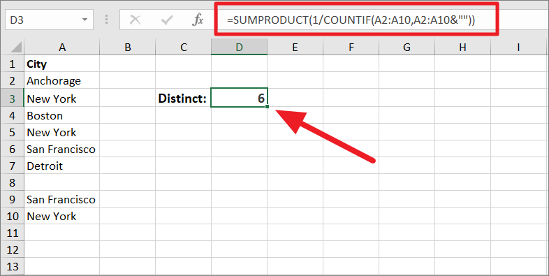
To include blank or empty cells in the count while counting distinct values, try the below formula:
=SUMPRODUCT(1/COUNTIF(A2:A10,A2:A10&""))As you can see above, when we concatenate an empty string (“”) to the data in the criteria argument of COUNTIF function, it returns 1 for an empty cell in the array of results: {1;4;1;4;2;1;1;2;4}. So the formula, 1/COUNTIF(A2:A10,A2:A10&"") = {1;0.25;1;0.25;0.5;1;1;0.5;0.25}. Finally, the SUMPRODUCT function adds up all the numbers from the array and gives us distinct values – 6 which also includes the empty cell in the count.
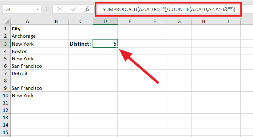
To ignore blank or empty cells from the count while counting distinct values, use the below formula:
=SUMPRODUCT((A2:A10<>"")/COUNTIF(A2:A10,A2:A10&""))Here, A2:A10<>"" produces a TRUE or FALSE array of results. When a cell is empty or blank in the range, it returns FALSE. So when the FALSE value is divided by any number, it returns 0. As a result, now this formula (A2:A10<>””)/COUNTIF(A2:A10,A2:A10&””) returns this array: {1;0.25;1;0.25;0.5;1;0;0.5;0.25}. When SUMPRODUCT sums up the array of results, you will get ‘5’ as the final count.
Two Way Lookup with SUMPRODUCT Function
Usually, you may use the INDEX and MATCH functions to lookup values in two dimensions, but in the earlier versions of Excel, the SUMPRODUCT was often used for two-way lookup and extraction. SUMPRODCUT is also perfectly capable of looking up values in two directions.
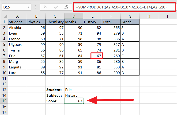
Let’s assume we have the below dataset where we want to look up and return Eric’s score in the History subject.
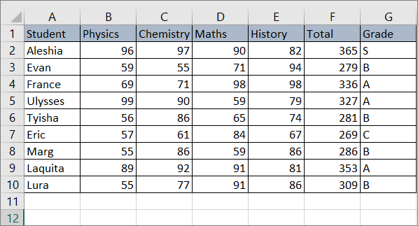
To perform a two-way lookup, write this SUMPRODUCT formula:
=SUMPRODUCT((A2:A10=D13)*(A1:G1=D14),A2:G10)In the formula, A2:A10=D13 looks for the value of cell D13 down the column A2:A10, and A1:G1=D14 looks for the value of cell D14 along the row A2:A10. Then, the SUMPRODUCT function returns the value at the intersection of the two look-ups, which is 67.
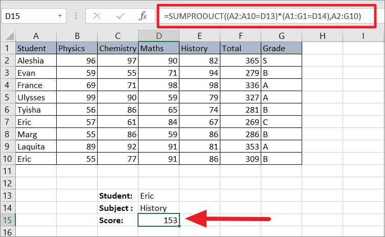
If there are multiple values satisfying the same condition, then the formula will return the sum of the returning values.
For example, if there are two Erics’ in the student names column, then the function will return the sum of both of their History scores:
Calculate the Weighted Average with SUMPRODUCT Function
Another common application of the SUMPRODUCT function is to calculate a weighted average where each value in a data set is assigned an identical weight. A weighted average is an average of a data set that takes into account the varying degrees of importance.
The syntax of SUMPRODUCT weighted average formula:
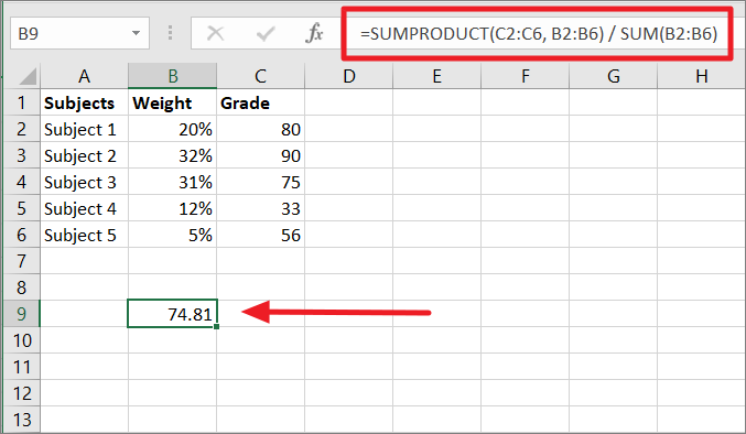
=SUMPRODUCT(values, weights) / SUM(weights)For example, let’s assume you have the below table of grade statistics in column B and their weight in column C.
=SUMPRODUCT(C2:C6, B2:B6) / SUM(B2:B6)In the above formula, you multiply each percentage (weight) with the corresponding grade and add those resulting product values together. After that, divide that sum of products number by the sum of five weights.
This is what the above formula looks like inside: =(B2*C2+B3*C3+B4*C4+B5*C5+B6*C6)/(B2+B3+B4+B5+B6)
SUMPRODUCT with IF function
You can combine the ‘SUMPRODUCT’ and the ‘IF’ function to sum values based on a condition.
Syntax:
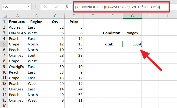
=SUMPRODUCT(IF(criteria_range=criteria, values_range1*values_range2))From the below data set we need to find the total sales of ‘Oranges’. To do that, we can use the below formula:
=SUMPRODUCT(IF(A2:A15=G3,C2:C15*D2:D15))After entering the formula, you need to press Ctrl+Shift+Enter simultaneously to apply this formula as an array formula.
The IF function checks for the value “Oranges” in the range A2:A15 and if it is found, it multiplies the corresponding values in columns C and D. Then, the Sumproduct function sums up all the product values.
SUMPRODUCT and IF with Multiple Criteria
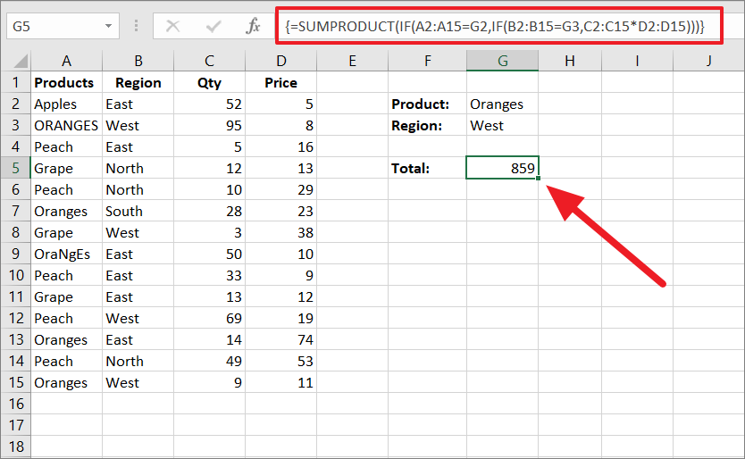
To find the total sales of Oranges from the West region, we need to add another criterion in the formula:
=SUMPRODUCT(IF(A2:A15=G2,IF(B2:B15=G3,C2:C15*D2:D15)))After typing the formula, make sure to press Ctrl+Shift+Enter to apply it as an array formula.
The first IF function in the SUMPRODUCT formula searches for the value entered in G2 (Oranges) in the range A2:A15. If the value is found, the second IF function checks for values entered in G3 (West) in the range B2:B15. And if both conditions are satisfied, the SUMPRODUCT multiplies the corresponding values in C2:C15 and D2:D15. In case any of the specified values are not found in the ranges, it will return FALSE.
As a result, we get this array of results – {FALSE;760;FALSE;FALSE;FALSE;FALSE;114;FALSE;FALSE;FALSE;1311;FALSE;FALSE;99. Here, FALSE means 0. Finally, the SUMPRODUCT function adds up the results to return – 859.
SUMPRODUCT with Other Functions
SUMPRODUCT function can be integrated with other functions to handle array functionality. Instead of entering long formulas and pressing Ctrl+Shift+Enter every time you want to run array formulas, you can use simply SUMPRODUCT to perform calculations on the arrays directly.
Example 1:
For instance, let’s assume you have a list of 5 different word or text strings in a range of A2:A6 and you want to count the total characters of all 5 text strings. Normally, you would add a helper column in column B and enter a LEN function like =LEN(A2), Then apply the same formula to B3, B4, B5, and B6 cells. Finally, you would use the SUM function to add all those results like =SUM(A2:A6).
However, with the SUMPRODUCT function, you can sum all the characters with a single formula with no extra helper column:
=SUMPRODUCT(LEN(A2:A6))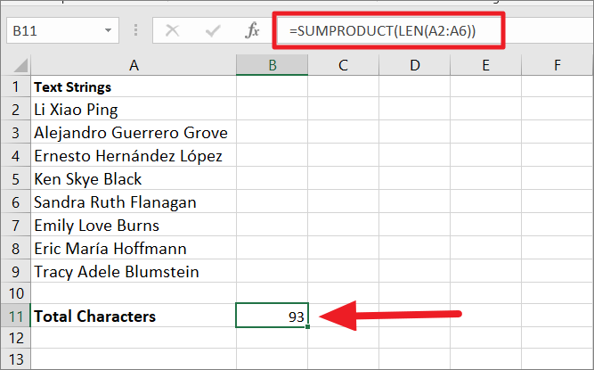
SUMPRODUCT with MONTH function
SUMPRODUCT can be used to sum or count values based on the month using the MONTH function.
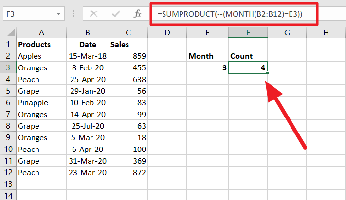
For example, we entered a month number into cell D2 and we want to count and sum the values for the specified month.
To count the number of sales in March, we can use the below formula:
=SUMPRODUCT(--(MONTH(B2:B12)=E3))Here, the MONTH function pulls the month from each date in B2:B12 and checks it against the specified month in E3. If it is equal, it returns TRUE, FALSE otherwise – {TRUE, FALSE, FALSE, FALSE, FALSE, FALSE, FALSE, TRUE, FALSE, TRUE, TRUE}.
Then, the double hyphen or negative converts the array into this: {1, 0, 0, 0, 0, 0, 0, 1, 0, 1, 1}. After that, the SUMPRODUCT aggregates the array to produce the number of march sales – 4.
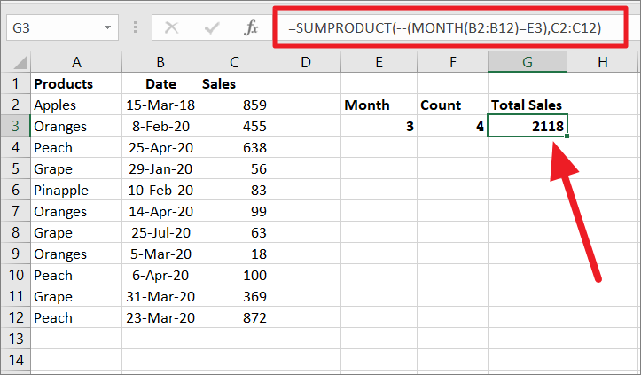
In case you want to find the total sales for the month of March, enter the below formula:
=SUMPRODUCT(--(MONTH(B2:B12)=E3),C2:C12)The MONTH function pulls the month from each date in B2:B12 and checks it against the specified month in E3. If it is equal, it returns TRUE, FALSE otherwise which is then converted to {1, 0, 0, 0, 0, 0, 0, 1, 0, 1,1}. Then, the SUMPRODUCT multiplies the resulting array with corresponding values in the Sales column (C2:C12) and adds up the product values to return the total sales of the march month – 2118.
SUMPRODUCT with ISNUMBER function
If you want to count the number of occurrences for specific words from a range of cells, you can combine SUMPRODUCT with ISNUMBER and FIND function to create a formula.
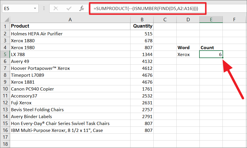
To count all the occurrences of words specified in cell D5, use the following formula:
=SUMPRODUCT(--(ISNUMBER(FIND(D5,A2:A16))))In the above formula, the FIND function looks for the text string entered in cell D5 (Xerox) in each cell of the range A2:A16. If the text string is found, the function returns the word’s starting position, otherwise, it returns an #VALUE! error.
After that, the ISNUMBER function returns TRUE if the FIND function produces a number, otherwise, it returns FALSE. Then, double negative converts the ISNUMBER results into this – {0, 1, 1, 0, 0, 1, 0, 1, 0, 0, 1, 0, 0, 0, 1}. At last, the SUMPRODUCT sums the array of results into – 6.
SUMPRODUCT with LARGE/SMALL function
The LARGE and SMALL function returns the nth largest and smallest numbers in a list of values when sorted by values in descending order or ascending order.
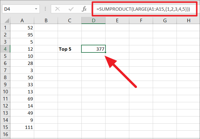
For instance, if you want to sum the top 5 largest values, try the below formula:
=SUMPRODUCT(LARGE(A1:A15,{1,2,3,4,5}))In the formula, the LARGE function returns the top 5 values from the list A1:A15. Usually, the LARGE function returns one nth largest value, but we enclosed {1, 2, 3, 4, 5} in double brackets. So, it returns all the 5 largest numbers – {111, 95, 69, 52, 49}. Then, the SUMPRODUCT formula adds those numbers into a sum – 377.
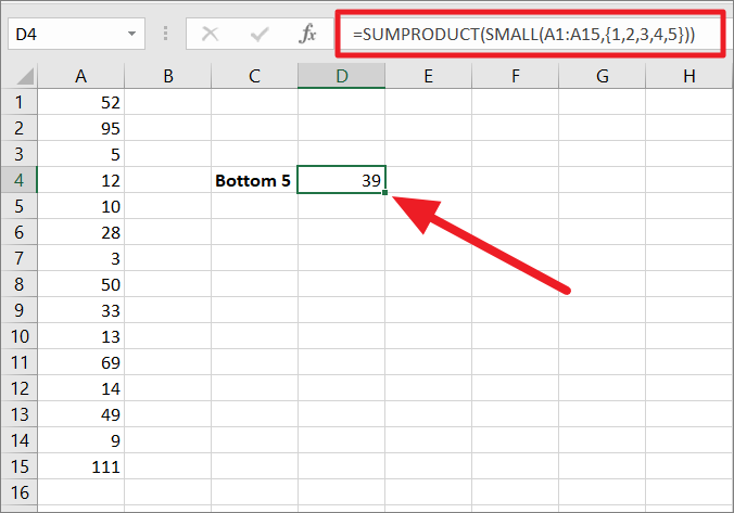
To sum the smallest 5 values, enter the below formula:
=SUMPRODUCT(SMALL(A1:A15,{1,2,3,4,5}))In the formula, the SMALL function returns the bottom 5 numbers of the range A1:A15. Usually, the SMALL function returns one nth largest values, but we enclosed {1, 2, 3, 4, 5} in double brackets. So, it returns all the 5 smallest numbers – {3, 5, 9, 10, 12}. Then, the SUMPRODUCT formula adds those numbers and outputs the sum of 5 smallest numbers – 39.
Compare Arrays with SUMPRODUCT
SUMPRODUCT function not only conditionally count, sum, average cells with multiple criteria from multiple columns, it can also compare two or more arrays.
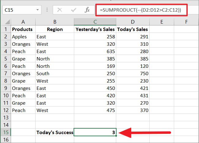
Suppose, you have the below table and you want to compare yesterday’s sales with today’s sales and figure out how many products have more sales today than yesterday. To do that, normally you have to compare column C against D and keep the score. But, with SUMPRODUCT, you can automate the process with a single formula. Let’s see how we can do that:
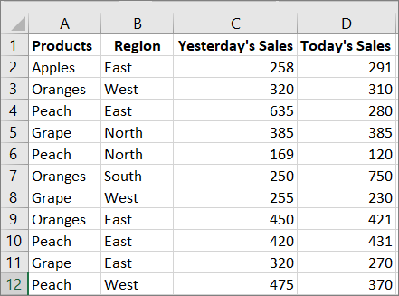
Here is a SUMPRODUCT formula that you can use to compare columns C and D:
=SUMPRODUCT(--(D2:D12>C2:C12))Here, we want to see if today’s sales are more than yesterday’s sales so we added the greater than (>) operator between the array arguments.
The formula checks each value of Today’s sales column against the corresponding value of Yesterday’s Sales column. If a value in the range D2:D12 is greater than the corresponding values in C2:C12, it returns TRUE; if not, returns FALSE. Then, double unary (–) converts those result into this array {1, 0, 0, 0, 0, 1, 0, 0, 1, 0, 0}. After that, all those values are added up and returned as the sum (3), which is the number of products that have sold more today than yesterday.
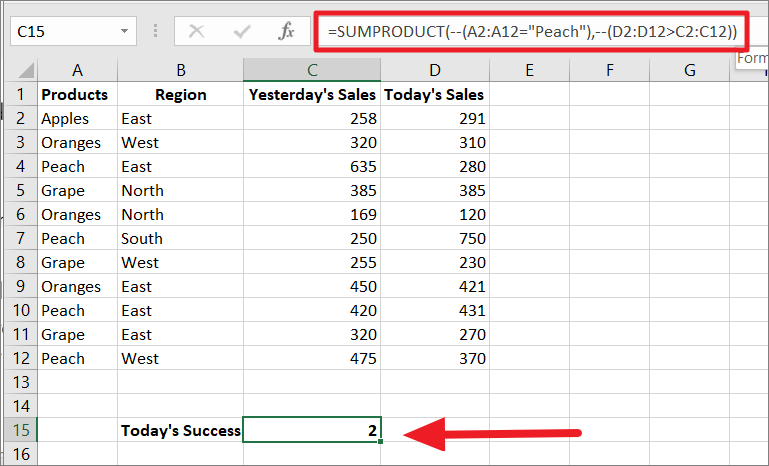
But what if you only want to see how many sales of Peach are higher than yesterday? Then, you have to another condition in the arguments:
=SUMPRODUCT(--(A2:A12="Peach"),--(D2:D12>C2:C12))The --(A2:A12=”Peach”) argument checks if the values ‘Peach’ is in the range A2:A12, and if it is in a cell, it return 1; if not, returns 0. This will create another array of results {0, 0, 1, 0, 0, 1, 0, 0, 1, 0, 1}.
=SUMPRODUCT({0, 0, 1, 0, 0, 1, 0, 0, 1, 0, 1}, {0, 1, 1, 0, 1, 0, 1, 1, 0, 1,1})
Then, the Sumproduct function multiplies the first array against their corresponding pair in the second array and adds up the product result to produce the output, which is 2. As you can see, there are only 2 times that today’s sales of Peach are higher than yesterday.
That’s it.