
Sometimes in Excel, you need to find the right input value that will produce a desired result in a formula. The Goal Seek feature simplifies this by calculating the necessary input to achieve your target output.
For example, imagine you’ve scored 75 marks in a subject but need a total of 90 to secure the highest grade. With one final test remaining, you want to know what score you must achieve to reach your goal. Goal Seek can help you determine the required score on that last test.
By iteratively testing different input values, Goal Seek quickly identifies the input needed to produce the desired output, saving you time compared to manual calculations.
Components of the Goal Seek Function
The Goal Seek feature in Excel requires three key components:
- Set cell – The cell containing the formula whose result you want to adjust.
- To value – The target value you want the formula to return.
- By changing cell – The cell that Excel will adjust to achieve the desired result.
Using Goal Seek in Excel: Example 1
Consider you own a fruit stall. In the spreadsheet below, cell B11 displays the cost of purchasing fruits ($1308), and cell B12 shows your total revenue from selling them ($1635). Cell B13 calculates your profit percentage, which is currently 20%.
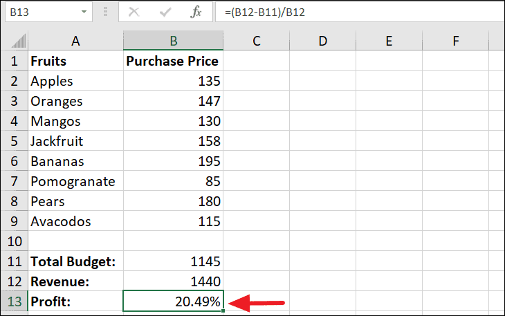
Suppose you aim to increase your profit margin to 30% without increasing your investment. This means you need to boost your revenue. But how much revenue is required to achieve a 30% profit? Goal Seek can help you find out.
Currently, you use the following formula in cell B13 to calculate the profit percentage:
=(B12-B11)/B12To determine the required revenue to reach a 30% profit margin, you can use Goal Seek by following these steps:
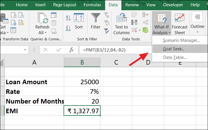
What-If Analysis button in the Forecast group and select Goal Seek from the dropdown menu.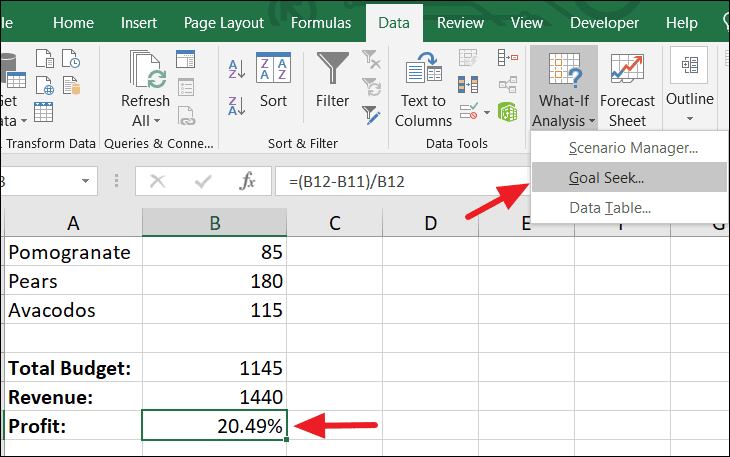
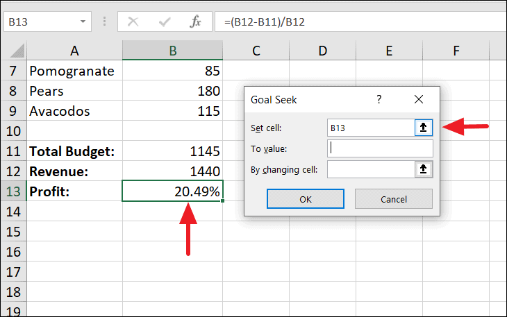
The Goal Seek dialog box will appear, prompting you to fill in three fields:
Set cell: Enter cell B13, which contains the formula you want to set to a specific value.
To value: Input the target profit percentage 0.30 (representing 30%).
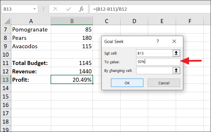
By changing cell: Specify cell B12, which is the revenue value that Excel can adjust to achieve the desired profit percentage.
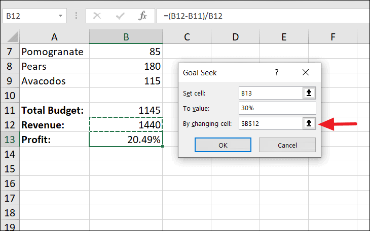
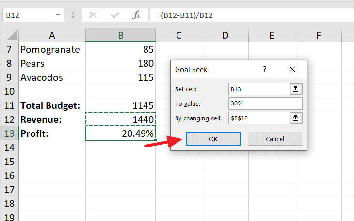
After entering the parameters, click OK to proceed.
Excel will adjust the value in cell B12 to meet your target profit percentage. A dialog box will inform you if a solution has been found.
In this case, Excel determines that increasing the revenue to $1,635.50 will result in a 30% profit margin.
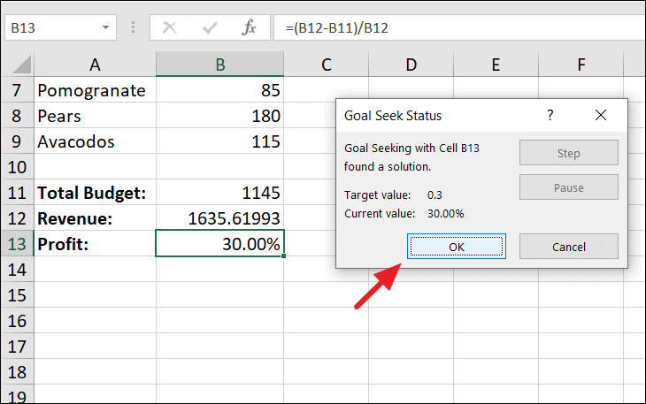
Click OK to accept the solution, and the cell values will update accordingly. Now, cell B12 displays the new revenue amount, and cell B13 reflects the updated profit percentage of 30%.
Things to Remember When Using Goal Seek
- The Set cell must contain a formula that depends on the By changing cell.
- Goal Seek can adjust only one variable at a time.
- The By changing cell must contain a numeric value, not a formula.
- If Goal Seek cannot find an exact solution, it will provide the closest possible value and notify you.
What to Do When Excel Goal Seek Is Not Working
If Goal Seek doesn’t find a solution but you believe one exists, try the following steps to resolve the issue.
Check Goal Seek Parameters and Values
Ensure that the Set cell refers to the correct formula cell and that this formula depends on the By changing cell, either directly or indirectly.
Adjust the Iteration Settings
You can modify Excel’s calculation settings to increase the number of iterations and improve the accuracy of results.
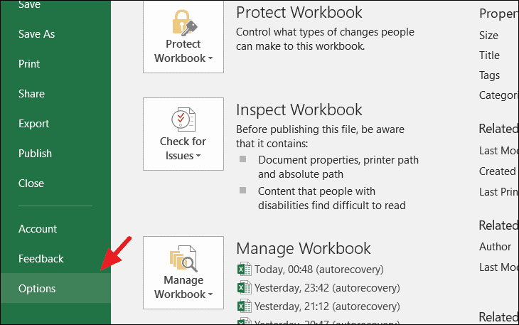
Maximum Iterations and Maximum Change values. Increasing Maximum Iterations allows Excel to test more solutions, and decreasing Maximum Change enhances accuracy.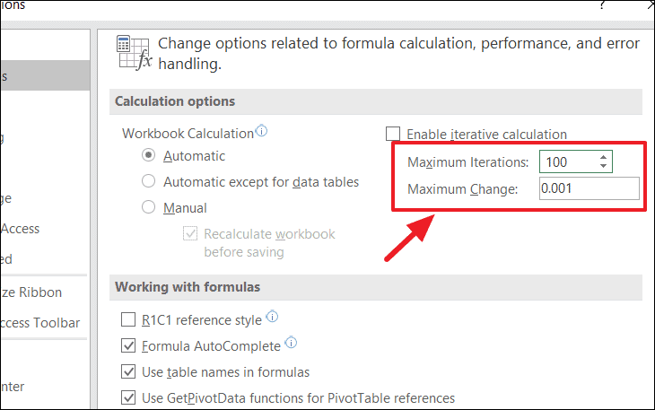
Avoid Circular References
Ensure that your formulas do not contain circular references, where a formula refers back to its own cell. Circular references can interfere with Goal Seek’s ability to find a solution.
Using Goal Seek in Excel: Example 2
Suppose you plan to borrow $25,000 at an interest rate of 7% per month over 20 months. This results in a monthly payment (EMI) of $1,327.97. However, you can only afford to pay $1,000 per month. Goal Seek can help you determine the maximum loan amount you can borrow while keeping the monthly payment at $1,000.
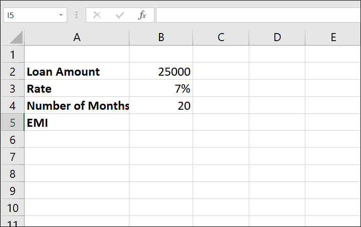
First, input the known variables into your spreadsheet:
- Principal (Loan Amount): $25,000 in cell B2.
- Interest Rate: 7% in cell B3.
- Term: 20 months in cell B4.
Next, use the PMT function in cell B5 to calculate the EMI:
=PMT(B3/12, B4, -B2)This formula computes the monthly payment based on the interest rate, term, and principal amount.
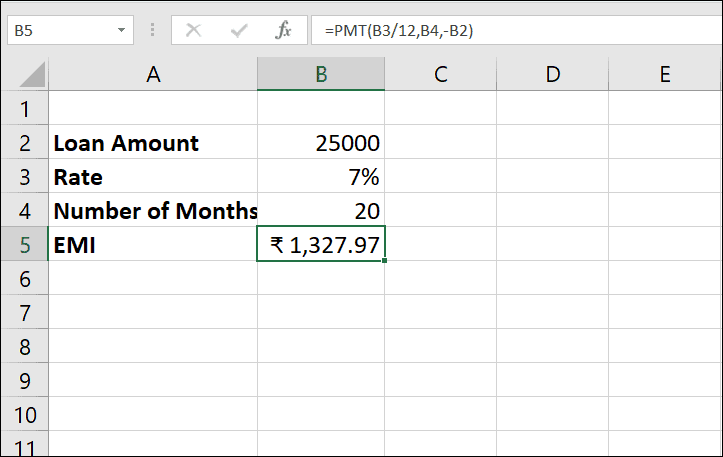
Currently, the EMI is calculated as $1,327.97.
Set cell: B5 (the cell with the EMI formula).
To value: -1000 (since the PMT function returns payment amounts as negative values).
By changing cell: B2 (the loan amount).
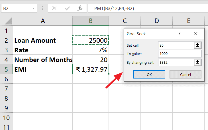
Click OK to run Goal Seek.
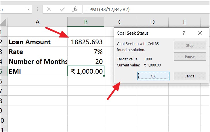
Excel adjusts the loan amount to find the maximum you can borrow while keeping the monthly payment at $1,000. The analysis shows that you can afford a loan amount of approximately $18,825 under these conditions.
Utilizing Excel’s Goal Seek feature allows you to efficiently find the necessary input values to achieve specific goals in your calculations, streamlining decision-making processes and complex computations.


