The IFERROR function is designed to handle errors resulting from formulas in Excel. The IFERROR function is a logical formula that is used to detect errors in formulas and returns an alternate value or performs another calculation in place of the error. If the formula nested inside the IFERROR function results in an error, the IFERROR function catches that error and returns a specified value in its place.
Excel shows errors whenever there’s something wrong with the formula or the cell it’s referencing, however, sometimes the error is unavoidable. Having an error not only makes your spreadsheet look bad but if another formula references the cell containing that error, (for instance when you sum a range of cells), it will cause another error in the second formula. So, rather than displaying an error, you can use the IFERROR function to return something else like zero, blank, or a text.
IFERROR function is an easy and elegant way to handle errors and keep your spreadsheets clean and your formulas transparent. Moreover, this function can be used in all the versions of Excel from Excel 2007. In this tutorial, we will learn what the IFERROR function is and how to use it to manage errors in Excel.
What is IFERROR Function in Excel?
The IFERROR function is a built-in function that returns a specified value if the formula nested in results in an error.
The Syntax of IFERROR function:
=IFERROR(value,value_if_error)The function has only two arguments:
value(required) – This is the value, expression, formula, or cell reference that is to be checked for errors. If the value or the result is an error it will return TRUE otherwise it will return FALSE.value_if_error(required) – This argument specifies what value to return or calculation to perform if an error is found. It could be anything a text string, a numeric value, an empty string (blank cell), another formula, expression, or calculation. If you specify a text string, you must enclose it in double quotes (” ”).
Also, if there is no error is found, it will return the usual result of the formula or expression in the value argument.
You can use the IFERROR function to detect and handle various formula errors such as the following:
- #N/A.
- #VALUE!
- #REF!
- #DIV/0!
- #NUM!
- #NAME?
- #NULL!
Most of the time, when you encounter these errors you can resolve the issue by correcting the formula. But, occasionally, these errors are inevitable and you might be expecting them. So, to deal with these errors, you can use the IFERROR function to substitute a value or function for the error.
Don’t confuse the IFERROR function with another similar error checking function, the ISERROR function which is to be used to check for errors and return simple TRUE or FALSE.
How to Use IFERROR function
Let us see how to catch errors using the IFERROR function and return different kinds of values instead of errors with examples.
If Error, Then Return 0
If you encounter an error in your formula, you can use the IFERROR function to return ‘0’ instead of the error.
Example 1:
For instance, in the below example, we wanted to find out the average sales of different items, so we divided the Sales values in column A by the Qty (Quality) values in Column B.
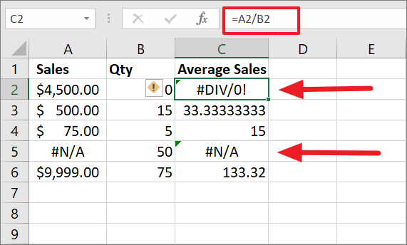
In the table, the Quantity value in B2 is 0, and the sales value in A5 is a #N/A (Not available) error. As a result, we ended up with #DIV/0! in C2 because when any number is divided by 0 (divisor), Excel throws the #DIV/0! error. And when #N/A error is divided by 50, it outputted another #N/A error in return.
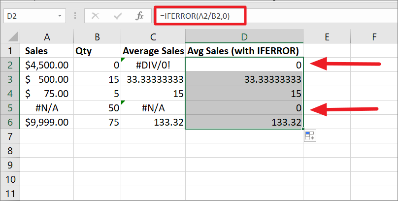
With the help of the IFERROR function, we can return ‘0’ as a result instead of displaying the error codes.
To handle the errors, you can nest the formula inside the IFERROR function:
=IFERROR(A2/B2,0)In the below example, we combined the IFERROR function with the same formula and entered it in a separate column. The above formula is entered in cell D2 and copied down to the whole column using the fill handle. As you can see below, the formula returns ‘0’ as the Average sales price when it detects an error.
Example 2:
If you ignore the second argument in the IFERROR function, the formula will return ‘0’ by default.
=IFERROR(A2/B2,)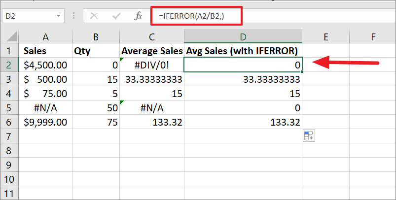
If Error, Then Return Blank
Instead of substituting 0 for errors, you specify an empty string (“) in value_if_errorargument of the IFERROR to return a blank cell if the result is an error.
Example 1:
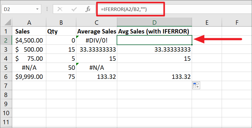
To return a blank cell if an error is found, use the below formula:
=IFERROR(A2/B2,"")In the formula, we entered double quotations (“”) which means an empty string to return a blank cell.
Example 2:
You can also use any symbol to replace an error instead of an empty cell using the IFERROR function.
To return a symbol or a character if an error is found, use the following formula:
=IFERROR(A2/B2,"-")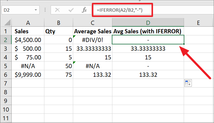
If Error, Then Show a Message/Text String
Instead of showing 0 or blank or an error, you can display your own message using the IFERROR function. When you add a text string in the second argument of the IFERROR function, make sure to enclose it in double quotes.
For example, this formula will return a message “Invalid input” instead of the error code:
=IFERROR(A2/B2,"Invalid Input")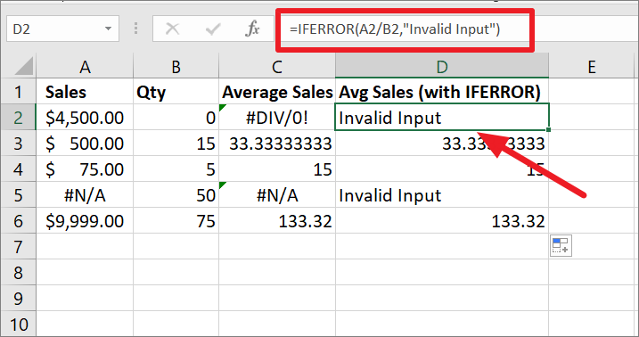
If Error, Then Perform a Calculation
With the IFERROR function, you can perform a second calculation if the first formula is evaluated to an error. You can achieve this by inputting the second formula in thevalue_if_error argument of the IFERROR.
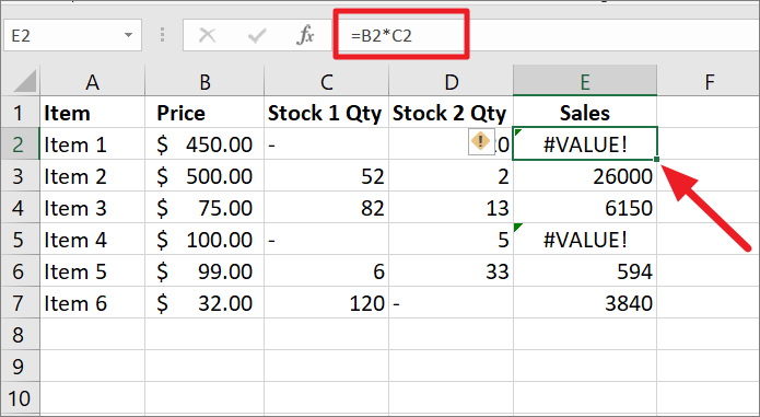
For instance, we want to find the sales of Stock 1 by multiplying the price of an item with Stock 1 quantity. However, we have no stock of two items, so when the price is multiplied by the dash (-) symbol, we get the Value error.
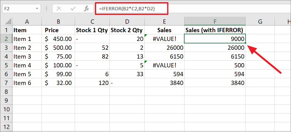
So if multiplying stock 1 quantity with price results in an error, multiply the stock 2 quantity with the price to find the sales amount of each item:
=IFERROR(B2*C2,B2*D2)In the above formula when multiplying B2 with C2 produces an error, the IFERROR function multiplies the B2 with D2 and returns the sales amount. If the first formula inside the IFERROR function didn’t result in an error, it returns that result.
IFERROR with Array Formulas
The array formula is used to perform multiple calculations in an array through a single formula. But sometimes, the Array formulas can also result in errors.
For example, we want to find the total average sales for the below table by dividing the value in column A by a value in column B in each row and summing up the results. But when we use the below array formula, it results in an error:
=SUM(A2:A6/B2:B6,0)The above formula divides each cell value in the range A2:A6 by the corresponding cell value of the range B2:B6 and returns array this array of results {#DIV/0!,33.33,15,#N/A,133.32}. Then the SUM function sums up the array of results to produce total average sales which also results in an error.
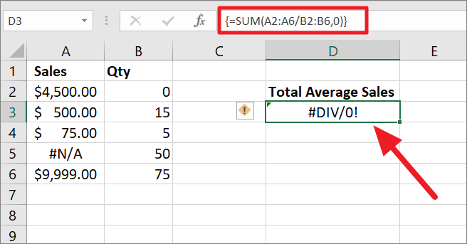
The formula divides the values in A2 by 0 and the error in A5 by the B5 which results in two errors. And when that two error values are added up with other values, we get an #DIV0! error.
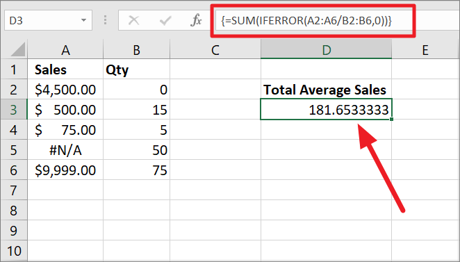
To solve this problem, you just need to enclose the division operation within the IFERROR function and then wrap the IFERROR function with the SUM function:
=SUM(IFERROR(A2:A6/B2:B6,0))To execute the array formula, press Ctrl+Shift+Enter.
The IFERROR function traps all the errors and replaces them with 0, creating this array of results – {0,33.33,15,0,133.32). Then, the SUM function adds up all the results and returns ‘181.65’.
IFERROR with VLOOKUP function
The IFERROR function is often combined with the VLOOKUP function to return a custom message or text if the search value does not exist in the data set.
VLOOKUP function searches for a value in the first column of a table or a range and extracts the corresponding value from a column to the right. However, if the lookup value is not found in the table or misspelled, you will get an #N/A! error in return. So to tidy up your spreadsheet, you can use the IFERROR function to return your own message instead of the errors.
Example:
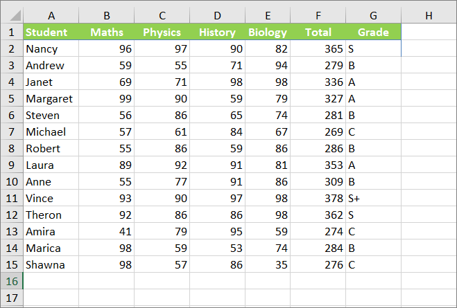
Suppose you have the below data, where you want to look up a student’s name and extract his/her score from a specific subject.
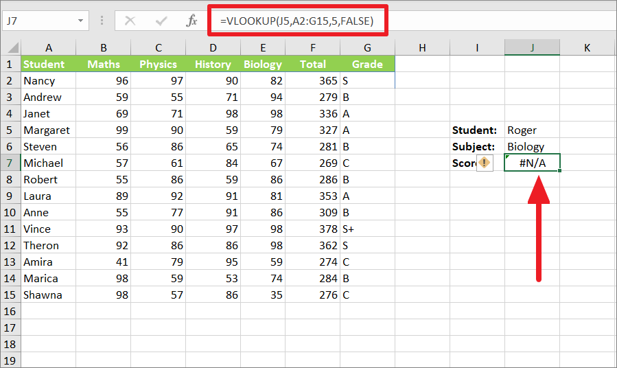
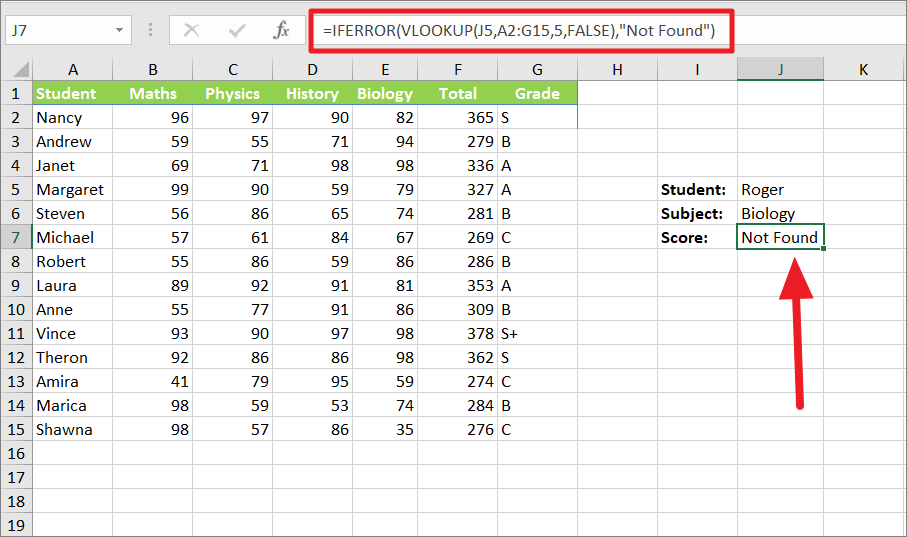
To look up a student named ‘Roger’ (J5) and return his biology score, we can use the below formula:
=VLOOKUP(J5,A2:G15,5,FALSE)However, the above this ends up with an error because the lookup value in cell J5 ‘Roger’ is not found in the table. Here, the first argument J5 specifies the lookup value, A2:G15 represents the range, 5 tells the function to retrieve the values from the fifth column, and FALSE means the search for the exact value.
If the value is not found, you can use the IFERROR function to return a custom text string like “Not found” or “wrong input” in case of an error. To do that, you have to wrap the VLOOKUP formula as the first argument and the text string you want to return as the second argument within the IFERROR formula.
To return a custom text string, if the VLOOKUP function evaluates to an error, enter the below formula:
=IFERROR(VLOOKUP(J5,A2:G15,5,FALSE),"Not Found")The above formula looks for the value ‘Roger’ (J5) in the range ‘A2:G15’ and generates an #N/A error because the value is not found in the table. However, the IFERROR function catches that error and returns the specified string “Not Found” in its place.
If the nested VLOOKUP function does not result in an error, then the IFERROR function will simply return the standard result of the VLOOKUP function.
For example, if you change the lookup value to ‘Robert’ instead of ‘Roger’, you will get the below result:
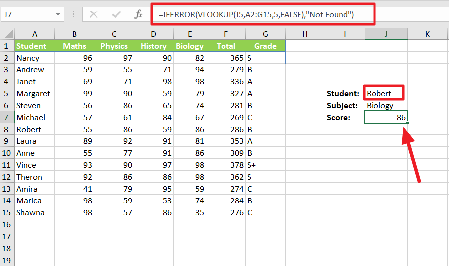
Here, we used the same formula but only changed the input value for the formula to ‘Robert’. As a result, we get the score ’86’ for the Biology subject.
IFERROR Function to Perform Sequential Vlookups
The IFERROR function can also be used to perform multiple Vlookups or sequential Vlookups based on whether the preceding lookup has resulted in an error or not.
Let’s assume you have a list of students’ scores in various subjects for Class 1 and Class 2 and you want to extract a specific student’s test score in a certain subject from class 1 using Vlookup.
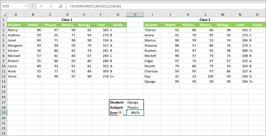
However, if the student you are searching for is not found in Class 1, you would end up with an error. So, if you nest two VLOOKUP functions (one for Class 1 and another for Class 2) as the two arguments of the IFERROR function, it performs the 2nd Vlookup operation and returns the results if the first VLOOKUP results in an error.
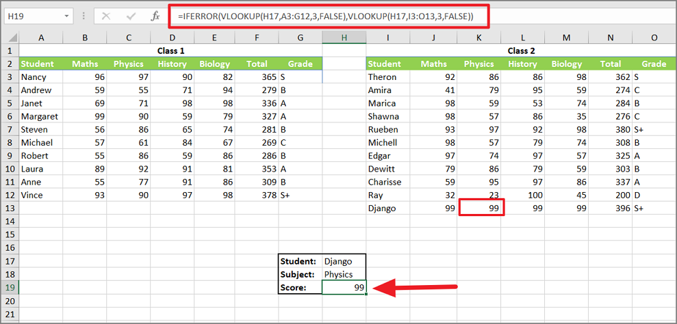
To do sequential VLOOKUPs with IFERROR, use the below formula:
=IFERROR(VLOOKUP(H17,A3:G12,3,FALSE),VLOOKUP(H17,I3:O13,3,FALSE))In the above formula, the first Vlookup function looks for the value in H17 (Django) by searching the array A3:G12 (Class 1) and if the lookup value is found, it returns the corresponding value in column 3 (Physics score). If the first VLOOKUP couldn’t find the value in Class 1, then it proceeds to the second Vlookup which searches for the values in the range I3:O13 (Class 2) and returns the Physics score for the student Django.
Nested IFERROR functions for Sequential Vlookups
However, what if the second Vlookup is also not able to find the lookup value and fails in the above formula, then we will get an error. To prevent this, you have to create a formula to return a custom message, if the lookup value is not found in both arrays.
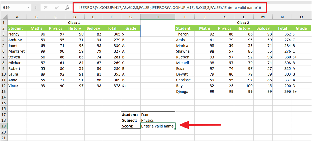
You need to create an IFERROR formula with the first VLOOKUP as the first argument (value) and another IFERROR function as the second argument (value_if_error). Then, nest the second VLOOKUP and a value_if_error message within the second IFERROR function:
=IFERROR(VLOOKUP(H17,A3:G12,3,FALSE),IFERROR(VLOOKUP(H17,I3:O13,3,FALSE),"Enter a valid name"))The first Vlookup inside the 1st IFERROR looks for the value ‘Dan’ in the array A3:G12 and if it fails, the second Vlookup inside the 2nd IFERROR looks for the value ‘Dan’ in the range I3:O3. If it also fails, the 2nd IFERROR returns the specified message “Enter a valid name”.
IFERROR with INDEX MATCH function
INDEX and MATCH function is a powerful lookup function more advanced than the VLOOKUP function that lets you search for a specific value in a range of cells and return a value at the specified row and column intersection.
Just like with VLOOKUP, if the INDEX MATCH function cannot find the lookup in the given range, it will return the error message. In such cases, we can use the IFERROR function to produce an alternate message or look up the value in another range by nesting the INDEX MATCH function.
Example:
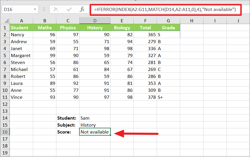
=IFERROR(INDEX(A2:G11,MATCH(D14,A2:A11,0),4),"Not available")In the above formula, the MATCH function tries to find the position of the lookup value in the range A2:A11, but the lookup value is not found in the array so the IFERROR returns the given alternate string “Not available”.
IF And IFERROR function
You can also combine the IFERROR function with the IF function to create an advanced formula and handle errors.
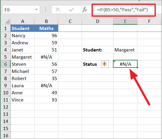
For example, we want to check whether the student Margaret is passed or failed using the IF function in the table. But Margaret’s score is not available in the table, so we get the #N/A error as the result.
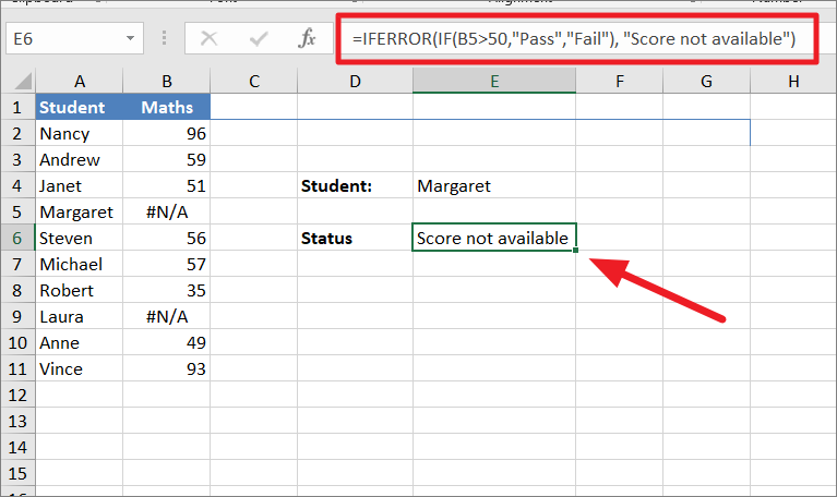
To fix this, we can use the below IF and IFERROR function combination:
=IFERROR(IF(B5>50,"Pass","Fail"),"Score not available")Here, the IF function checks whether the value in B5 is greater than 50 and returns an error. Then, the IFERROR function traps that error and displays the given alternate text string instead.
IFERROR vs. ISERROR
ISERROR function is another error-handling function that is used to check if a formula evaluates to an error or not and return TRUE or FALSE as a result. The IFERROR function returns an alternate value if a formula results in an error.
Syntax of ISERROR:
=ISERROR(value)ISERROR function (logical condition) is often used with the IF function to execute an operation or return a value if the logical condition results in an error and what to do if doesn’t result in an error.
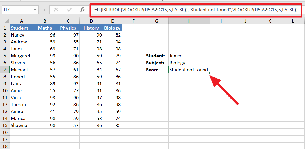
For example, we want to extract Janet’s marks in Biology using this IF ISERROR formula:
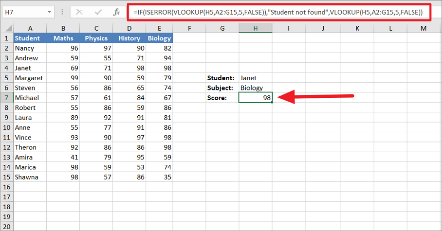
=IF(ISERROR(VLOOKUP(H5,A2:G15,5,FALSE)),"Student not found",VLOOKUP(H5,A2:G15,5,FALSE))Here, the ISERROR checks whether the nested Vlookup formula results in an error or not. If it is TRUE, then the IF function returns the message “Student not found”, otherwise it performs the Vlookup function again and returns the score ’98’.
If the lookup value (student) is not found:
or, if the student name is found:
IFNA vs. IFERROR
IFNA is another error checking function that is similar to the IFERROR that is used to catch only #N/A errors while IFERROR handles all error types. IFNA formula is useful if you only want to return a customized response for a #N/A error but not for all other errors.
Syntax of IFNA Function:
IFNA(value, value_if_na)value– the value, expression, formula, or cell reference that is to be checked for errors.value_if_na– represents what value to return or calculation to perform in case of an #N/A error. It could be anything a text string, a numeric value, empty string (blank cell), another formula, expression, or calculation.
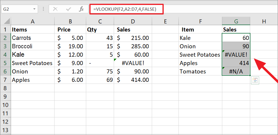
Suppose, you have the below table of sales reports and you want to pull the Sales amount of a few items from the table. To do that, we are using this simple VLOOKUP formula:
=VLOOKUP(F2,$A$2:$D$7,4,FALSE)The above formula is entered in cell G2 and the same formula is applied to the range G2:G6 using the fill handle. When we do that, we get a #VALUE! and a #N/A error for two items.
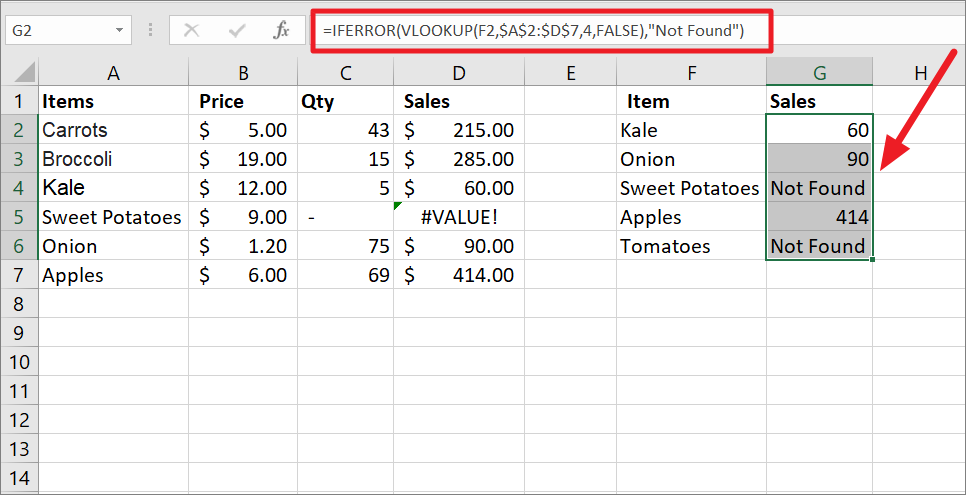
To handle these errors, you can nest the above VLOOKUP formula inside the IFERROR function:
=IFERROR(VLOOKUP(F2,$A$2:$D$7,4,FALSE),"Not Found")This IFERROR formula will handle all the errors and return the “Not Found” message whenever there’s an error is found. The above formula is applied to the whole range G2:G6.
But we don’t want that, we only want to show the “Not found” message for the items that don’t exist in the table (Tomatoes). That means, we only need to catch and handle the #N/A errors which only appear if the lookup value is not present in the lookup table. To do that, we have to nest the VLOOKUP function inside the IFNA function.
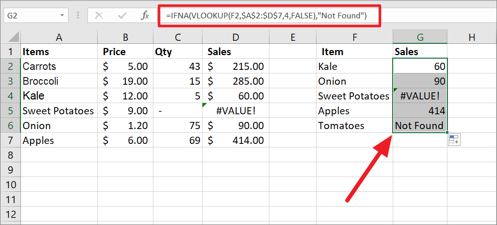
To catch only #N/A errors, use the below formula:
=IFNA(VLOOKUP(F2,$A$2:$D$7,4,FALSE),"Not Found")The above formula is applied to the range G2:G6. It checks the VLOOKUP function only for the #N/A error and returns the text “Not Found” if the item is not found in the table. As you can see below, it only catches the #N/A that occurs in cell G6 and returns the message. And it does not catch the #VALUE! error that occurs in cell G4 and displays the error as it is.
That’s it.


