
Excel formulas allow users to automate expiry date calculations, eliminating manual tracking errors and saving significant time for inventory, product shelf-life, or certification management. Calculating expiry dates in Excel can be accomplished using built-in date functions, arithmetic, and conditional formatting. The following sections detail the most effective methods, ranging from straightforward formula-based approaches to advanced conditional formatting for visual tracking.
Method 1: Using the EDATE Function for Expiry Date Calculation
The EDATE function directly adds a specified number of months to a given date, making it the most streamlined approach for typical expiry scenarios such as product shelf-life or membership renewals.
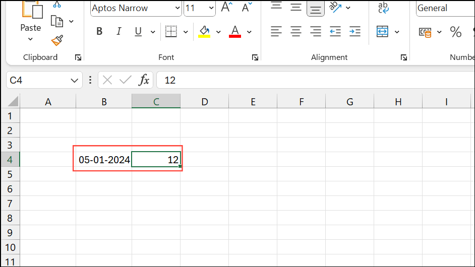
Step 1: Enter your start date (e.g., manufacturing or purchase date) in one column. In a second column, input the number of months until expiry. For example, if your start date is in B4 and the expiry period in months is in C4, the expiry date will be calculated in D4.
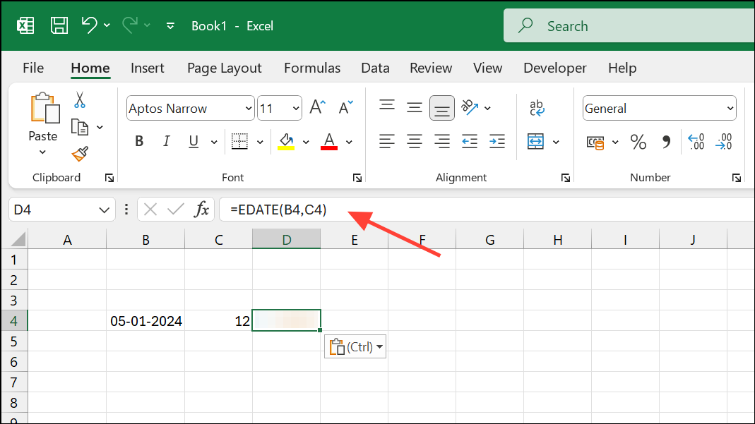
Step 2: In the expiry date cell, use the following formula:
=EDATE(B4,C4)This formula adds the number of months in C4 to the date in B4. Drag the formula down to apply it to other rows as needed.
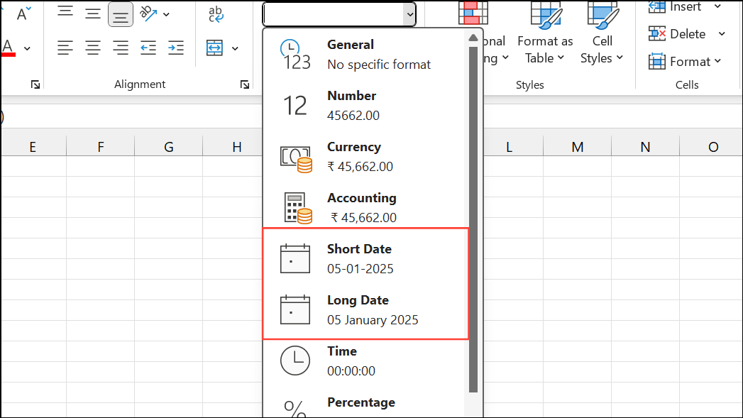
Step 3: If the result displays as a number, format the cell as a date. Select the cell(s), go to the Home tab, and choose "Short Date" or "Long Date" from the Number Format dropdown.
This method is reliable for most expiry calculations based on months.
Method 2: Calculating Expiry Dates with Days, Weeks, or Years
For expiry periods defined in days, weeks, or years, simple date arithmetic or the DATE function is effective.
- Days: Add the number of days directly to the start date.
=B3+45(for 45 days after the date inB3) - Weeks: Multiply weeks by 7 and add to the start date.
=B3+10*7(for 10 weeks after the date inB3) - Years: Use the
DATEfunction to add years.=DATE(YEAR(B3)+2,MONTH(B3),DAY(B3))(for 2 years after the date inB3)
These formulas can be adapted for any starting cell and expiry interval. Always format the output cells as dates for clear results.
Method 3: Handling Complex Expiry Rules (e.g., Certification Scenarios)
Some business rules require expiry dates based on conditional logic, such as certifications that expire two years after training if completed January–June, or three years if completed July–December, always expiring on December 31 of the relevant year.
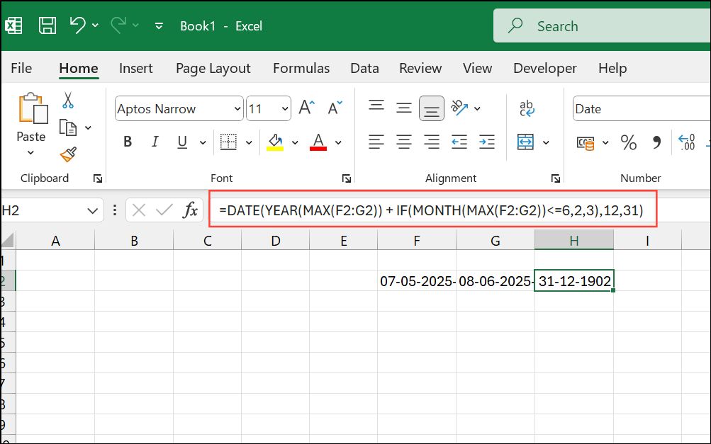
To automate this, use a formula that checks the month and selects the latest relevant date (e.g., recertification if available, otherwise the original training date). Assuming training date is in F2 and recertification date in G2, place the following formula in the expiry date column (H2):
=DATE(YEAR(MAX(F2:G2)) + IF(MONTH(MAX(F2:G2))<=6,2,3),12,31)This formula works by:
- Using
MAX(F2:G2)to select the latest date (recertification if present). - Checking the month with
MONTH()and adding 2 or 3 years as required. - Constructing the expiry date as December 31 of the calculated year.
Drag the formula down to apply it to the entire column. Adjust cell references as needed for your sheet layout.
Method 4: Calculating Time Remaining Before Expiry
To monitor how much time remains before an expiry date, subtract the current date from the expiry date. You can use the TODAY() function to always use the current date.
For example, if the expiry date is in C5:
=IF(C5>TODAY(),C5-TODAY()&" days","Expired")This formula displays the number of days left if the expiry date is in the future, or "Expired" if the date has passed. For a more detailed breakdown (years, months, days), use the DATEDIF function:
=IF(C5>TODAY(),
DATEDIF(TODAY(),C5,"y")&" years, "&
DATEDIF(TODAY(),C5,"ym")&" months, " &
DATEDIF(TODAY(),C5,"md")&" days",
"Expired")
This formula outputs the remaining time in years, months, and days until expiry.
Method 5: Highlighting Expiry Dates with Conditional Formatting
Visual tracking of expiry dates can be optimized using conditional formatting, which automatically changes cell colors based on how close the date is to expiry.
Step 1: Select the column or range containing expiry dates.
Step 2: Go to the Home tab, click "Conditional Formatting," and choose "New Rule."
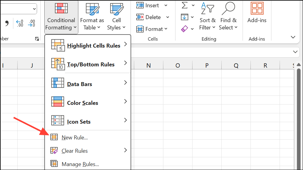
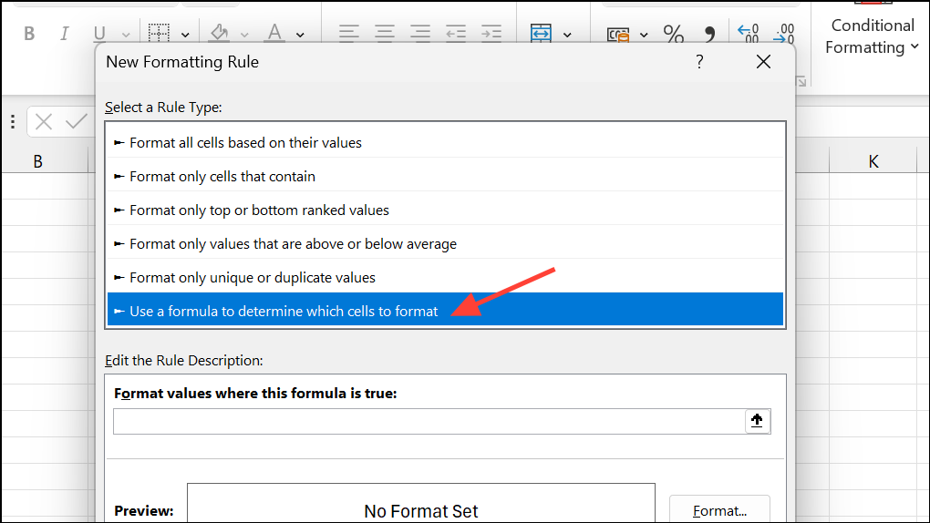
Step 3: Choose "Use a formula to determine which cells to format."
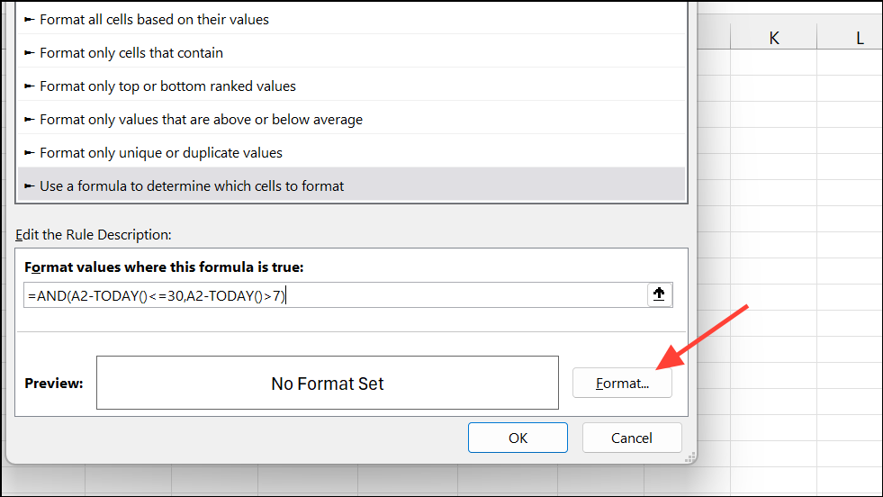
Step 4: Enter a formula such as:
- For yellow when expiry is within 30 days:
=AND(A2-TODAY()<=30,A2-TODAY()>7) - For red when expiry is within 7 days:
=A2-TODAY()<=7
Step 5: Click "Format," select the desired fill color, and click OK. Repeat to add multiple rules for different time frames (e.g., yellow for 30 days, red for 7 days).
This approach provides immediate visual cues for approaching or overdue expiries, allowing for faster decision-making and prioritization.
Automating expiry date calculations and tracking in Excel strengthens accuracy, saves time, and makes ongoing monitoring far more reliable. Regularly review your formulas and formatting rules to keep your tracking system working smoothly as your data grows.