How to Calculate Percent Change in Excel [Formula]

If you work with numbers a lot in your day-to-day work, you’ll often need to calculate percentages. Excel makes this real easy by helping you calculate different kinds of percentages using various formulas and methods. Calculating Percentages in an Excel sheet is similar to calculating in your school maths papers, it’s very easy to understand and use.

One of the most common percentage calculations people do in Excel is to calculate the percentage change between two values over a period of time. A Percentage Change or Percentage Variance is used to show the rate of change (growth or decline) between two values from one period to another. It can be used for financial, statistical, and many other purposes.

For example, if you want to find the difference between sales of last year and the sales of this year, you can calculate it with the percentage change. In this tutorial, we’ll cover how to calculate percentage change as well as a percentage increase and decrease between two numbers in Excel.

Calculating Percentage Change in Excel

Calculating Percentage Change between two values is an easy task. You just need to find the difference between two numbers and divide the result with the original number.

There are two different formulas you can use to calculate percentage change. Their syntaxes are as follows:

=(new_value – original_value) / original_value

=(new Value / original Value) – 1

new_value – is the current/final value of the two numbers you are comparing.
previous_value – is the initial value of the two numbers you are comparing for calculating percentage change.

Example:

Let’s take a look at this list of hypothetical fruit orders with column B contains the number of fruits ordered last Month and column C contains the number of fruits ordered this month:

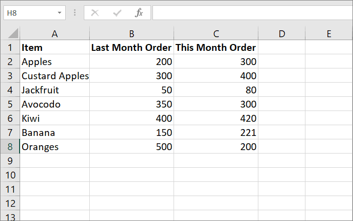
For example, you ordered a certain number of fruits last month and this month you ordered more than what you ordered last month, you can enter the below formula to find the percentage difference between the two orders:

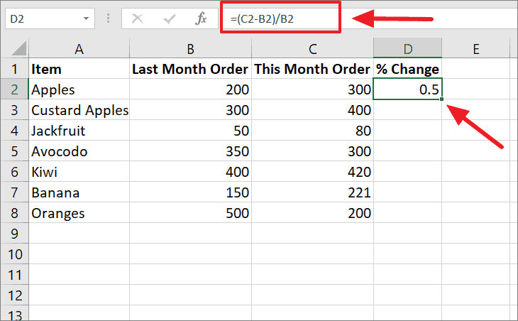
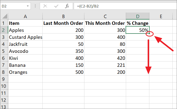
=(C2-B2)/B2

The above formula will be entered in cell D2 to find the percentage change between C2 (new_value) and B2 (original_value). After typing the formula in a cell, press Enter to execute the formula. You get the percentage change in decimal values as shown below.

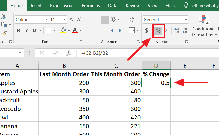
The result is not formatted as a percentage, yet. To apply percentage format to a cell (or a range of cells), select the cell(s), then click the ‘Percentage Style’ button in the Number group of the ‘Home’ tab.

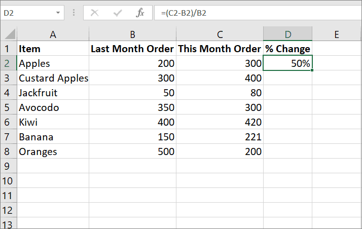
The decimal value will be converted to a percentage.

Calculate Percentage Change between Two Column of Numbers

Now, we know the percentage change between two orders for Apples, let’s find the percentage change for all the items.

To calculate the percentage change between two columns, you need to enter the formula in the first cell of the result column and AutoFill the formula down the whole column.

To do that, click the fill handle (the small green square at the lower right corner of the cell) of the formula cell and drag it down to the rest of the cells.

Now you got the percentage change values for two columns.

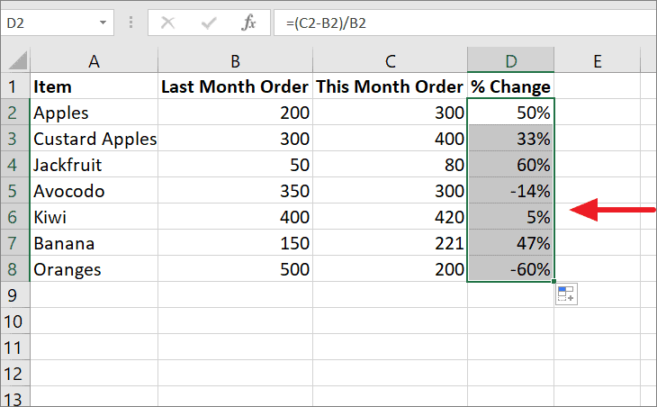
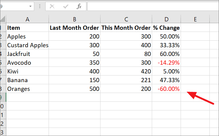
When the new value is higher than the original value, the result percentage would be positive. If the value new value is lower than the original value, then the result would be negative.

As you can see, the percentage change for ‘Apples’ is increased by 50%, so the value is positive. The percentage for ‘Avocodo’ is decreased by 14%, hence the result is negative (-14%).

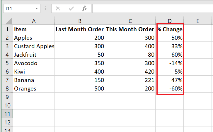
You can also use custom formatting to highlight the negative percentages in red color, so it can be easily identified when you are looking for it.

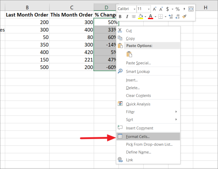
To format the cells, select the cells you want to format, right-click and select the ‘Format Cells’ option.

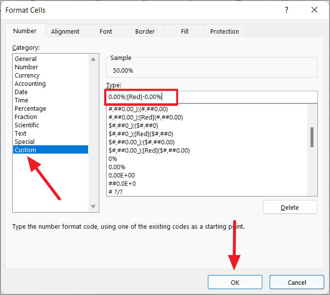
In the Format Cells window that appears, click on ‘Custom’ at the bottom of the left menu and type the below code in the ‘Type:’ text box:

0.00%;[Red]-0.00%

Then, click the ‘OK’ button to apply the formatting.

Now, the negative results will be highlighted in red color. Also, this formatting increases the number of decimal places to show accurate percentages.

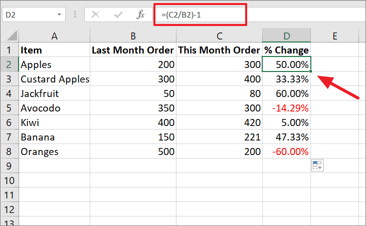
You can also use another formula to calculate percentage change between two values (Last Month Order and This Month Order):

=(C2/B2)-1

This formula divides the new_value (C2) by the original value (B2) and subtracts ‘1’ from the result to find the percentage change.

Calculating Percent Change Over Time

You can calculate period to period percentage change (month to month change) to understand the rate of growth or decline from one period to the next (for every month). This is very helpful when you want to know the percentage change for every month or year over a specific period of time.

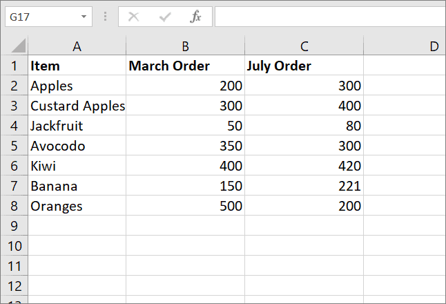
In the below example, we have the price of fruits for March month in column B and the price for July month, 5 months later.

Use this generic formula to find the percentage change over time:

=((Current_value/Original_value)/Original_value)*N

Here, N stands for the number of periods (years, months, etc.) between the two values of initial and current.

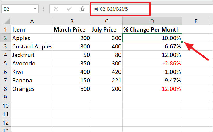
For example, If you want to understand the rate of inflation or deflation in prices for every month for over 5 months in the above example, you can the below formula:

=((C2-B2)/B2)/5

This formula is similar to the formula we used before, except, we need to divide the percentage change value by the number of months between two months (5).

Calculating the Percentage Growth/Change Between Rows

Let’s say you have one column of numbers that lists the monthly price of petrol for over a year.

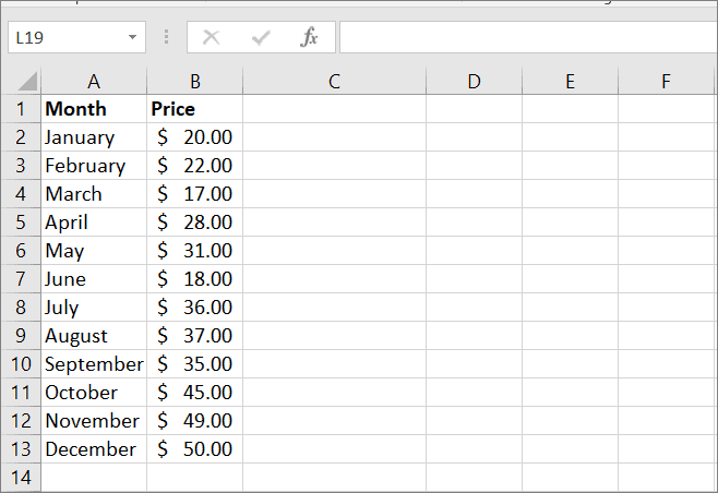
Now, if you want to calculate the percentage of growth or decline between rows so that you can understand the month-over-month changes in prices, then try the below formula:

=(B3-B2)/B2

Since we need to find the percentage of growth for February (B3) from the price of January (B2), we need to leave the first row blank because are not comparing January to the prior month. Enter the formula in cell C3 and press Enter.

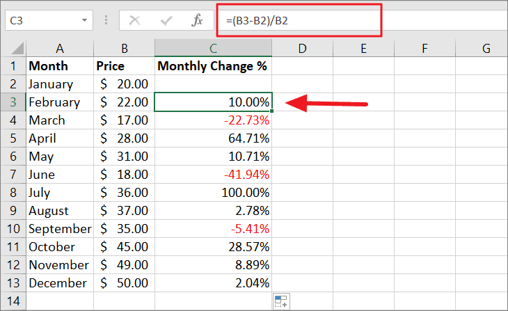
Then, copy the formula to the rest of the cells to determine the percentage difference between each month.

You can also calculate the percentage change for each month compared to January (B2). To do this, you need to make that cell an absolute reference by adding the $ sign to the cell reference, e.g. $C$2. So the formula would look like this:

=(B3-$B$2)/$B$2

Just like before, we skip the first cell and enter the formula in cell C3. When you copy the formula to the rest of the cells, the absolute reference ($B$2) doesn’t change, while the relative reference (B3) will change to B4, B5, and so on.

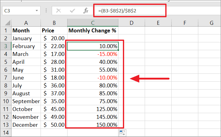
You will get a percentage rate of inflation or deflation for each month compared to January.

Calculating Percentage Increase in Excel

Calculating Percentage Increase is similar to calculating percentage change in Excel. Percentage Increase is the rate of the increase to the initial value. You will need two numbers to calculate the percentage increase, the Original number, and the New_number number.

Syntax:

Percentage Increase = (New_number - Original_number) / Original_number

All you have to do is subtract the original (first) number from the new (second) number and divide the result by the original number.

For example, you have a list of bills and their amounts for two months (April and May). If your bills for April month are increased in May month, then what is the percentage increase from April to May? You can use the below formula to find out:

=(C2-B2)/B2

Here, we subtract the May month electricity bill (C2) from the April month bill (B2) and divide the result by the April month bill. Then, copy the formula to other cells using the fill handle.

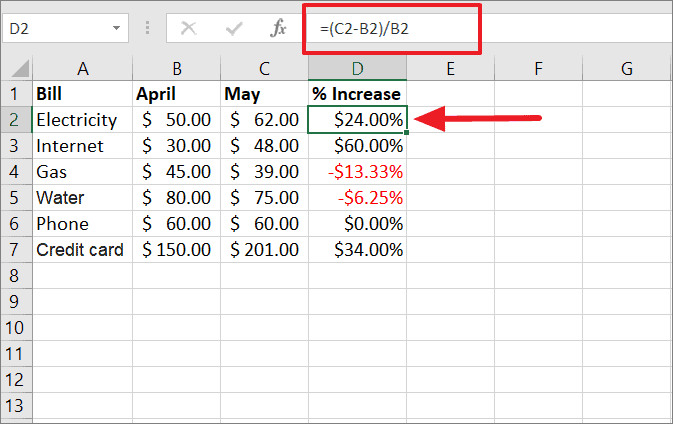
If you get a positive result ($24.00%), the percentage increased between the two months, and if you get a negative result (e.g. -$13.33%), then the percentage is actually decreased rather than increased.

Calculating Percentage Decrease in Excel

Now, let’s see how to compute the percentage decrease between numbers. The percentage decrease calculation is very similar to the percentage increase calculation. The only difference is that the new number will be smaller than the original number.

The formula is near identical to the percentage increase calculation, except in this, you subtract the original value (first number) from the new value (second number) before dividing the result by the original value.

Syntax:

Percentage Decrease = (Original_number - New_number) / Original_number

Let’s assume you have this list of storage devices and their prices for two years (2018 and 2020).

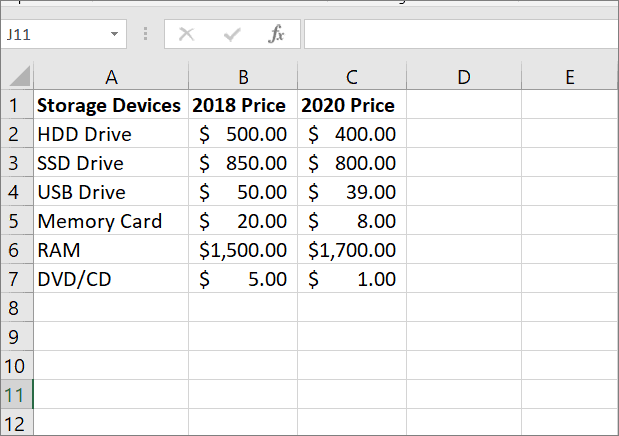
For example, the prices of storage devices were higher in the year 2018, and the prices were decreased in the year 2020. What is the percentage decrease of prices for 2020 compared to 2018? You can use this formula to find out:

=(B2-C2)/B2

Here, we subtract the 2018 price (B2) from the 2020 price (C2) and divide the sum by the 2018 price. Then, we copy the formula down to other cells to find the percentage decrease for other devices.

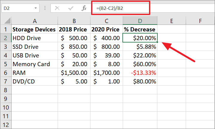
If you get a positive result ($20.00%), the percentage decreased between the two years, and if you get a negative result (e.g. -$13.33%), then the percentage is actually increased rather than decreased.

Common Errors You Get When Using the Above Formulas

When using the above formulas, you may occasionally run into this list of common errors:

#DIV/0!: This error occurs when you attempt to divide a number by zero (0) or by a cell that is empty. E.g. The value B6 in the formula ‘=(B6-C6)/B6’ is equal to zero, hence the #DIV/0! error.

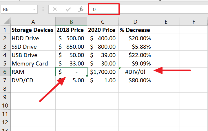
When you enter ‘zero’ in currency format, it will be replaced by dash (-) as shown above.

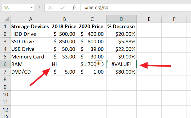
#VALUE: Excel throws this error when you’ve entered a value that is not a supported type or when cells are left blank. This often can occur when an input value contains spaces, characters, or text instead of numbers.

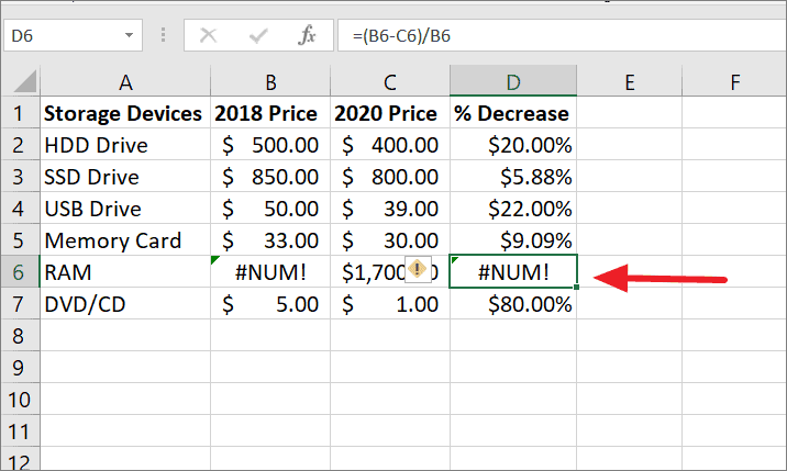
NUM!: This error happens when a formula contains an invalid number that results in a number that’s too large or too small to be shown in Excel.

Convert an Error to Zero

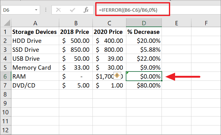
But there is a way we can get rid of these errors, and display ‘0%’ in its place when the error occurs. To do that, you need to use the ‘IFERROR’ function, which returns a custom result when a formula produces an error.

Syntax of IFERROR function:

=IFERROR(value, value_if_error)

Where,

value is the value, reference, or formula to check.
value_if_error is the value we want to display if the formula returns an error value.

Let’s apply this formula in one of the error examples (#DIV/0! error):

=IFERROR((B6-C6)/B6,0%)

In this formula, the ‘value’ argument is the percent change formula and the ‘value_if_error’ argument is ‘0%’. When the percent change formula encounters an error (#DIV/0! error), the IFERROR function would display ‘0%’ as shown below.