When working with a large spreadsheet, there are times when you may want to count the number of unique values in an Excel range. For instance, when you want to make a report of the number of customers who purchased your products only once or a number of students who only won in one event or remove duplicates from the order list and count only the unique items. Whatever the cases, it can be helpful to know how many unique values (or distinct) are in a column.
Although Excel does not have any pre-defined formula or options to count unique and distinct values, it is possible to count unique values in Excel using various methods. Unique values are the values that appear or occur only once in a list or column while distinct values are different values in a list that are unique values with at least 1 instance of duplicate value. In this article, we will share with you different ways of counting unique values in Excel.
Use Advanced Filter to Count Unique Values in Excel
The Advanced Filter method is one of the easiest methods for counting unique values in Excel which doesn’t involve any formulas. Follow these steps to count unique values using the Advanced filter feature in Excel.
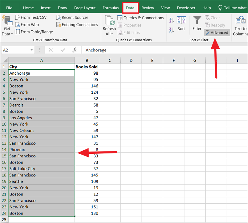
First, select the range of cells or select any of the cells is in the range from which you want to count unique values. Then, go to the ‘Data’ tab and click on the ‘Advanced’ option in the ‘Sort & Filter’ group.
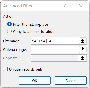
Once you do that, a small Advanced Filter dialog box will appear. Here, you have two options (Actions) – Filter the list and leave only the unique values in the selected range or filter the list and copy the unique values to another location leaving the source data intact.
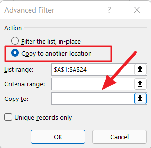
Now, select the ‘Copy to another location’ option. Then, click on the ‘Copy to’ field and select an empty cell or range where you want the filtered unique values.
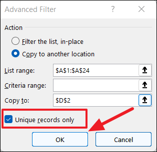
After that, select the ‘Unique Records Only’ checkbox and click ‘OK’.
However, if you want to replace the current list with the filtered unique values select the ‘Filter the list, in-place’ option under Action and click ‘OK’.
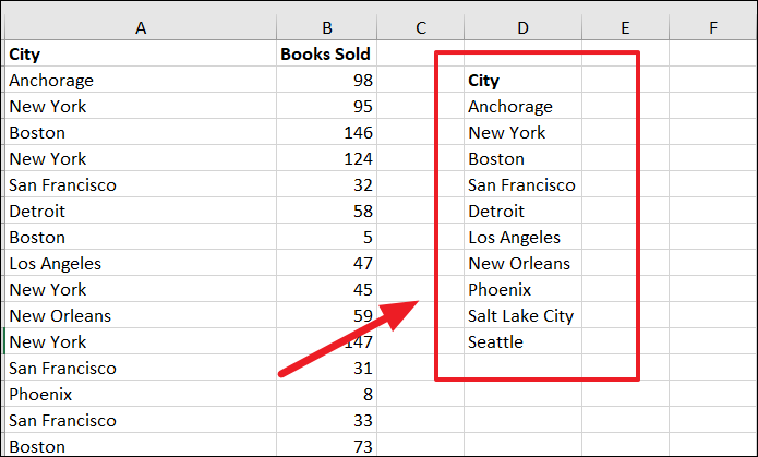
Either way, you will get a list of unique values from the source range as shown below.
To get the count of these unique values, select the cell below the list or an empty cell and enter the below formula:
=COUNTA(D3:D12)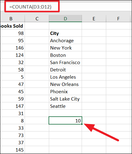
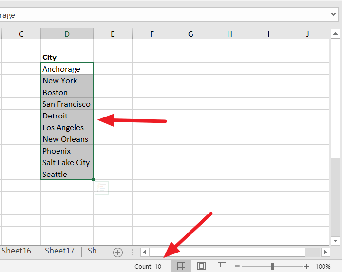
Alternatively, simply select the list of unique values and check your status bar at the bottom right corner of the Excel window (next to the zoom control). There, you will see the count of unique values as shown below.
Remove Duplicate Data to Get Unique Values
Another quick and easy way to get the count of unique values is to remove the duplicate values in a column and see how many values are left. Here’s how:
First, copy the data into a new sheet or a different column if you don’t want to lose the original data because removing duplicates will delete all the duplicate data and leave only the unique values.
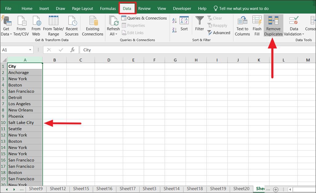
Then, select the range of cells or select any cell in that range that contains the values from which you want to remove duplicates, go to the ‘Data’ tab and select the ‘Remove Duplicates’ button in the Data Tools group.
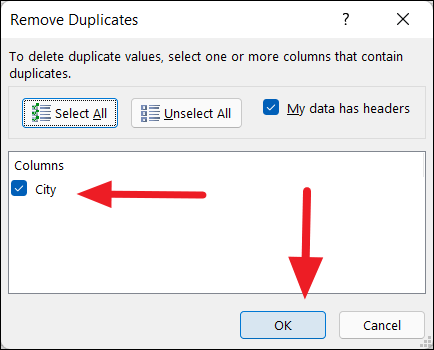
In the Remove Duplicates dialog box, select the column(s) from which you want to remove the duplicate values and click ‘OK’.
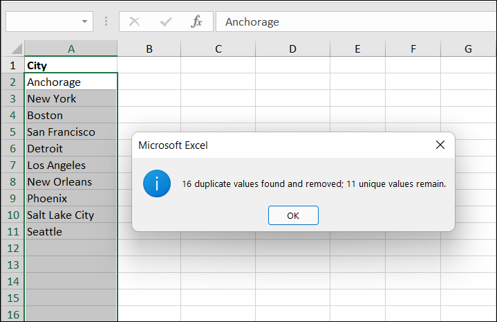
Once you click the ‘OK’, you will see a prompt box informing you how many duplicate values were removed and how many unique values are remaining.
If you want the unique value count in a cell, then you will need to the use COUNTA formula from the above method.
However, the problem with this method is that it not only filters unique values (occurring only once), but it removes duplicates for values that occur multiple times and leaves only one instance of those values. If you only want to count unique values, then you have to combine several Excel functions.
Counting Distinct Values using Formulas in Excel
We have seen how to count unique values using Excel options, now let us see how to count unique and distinct values using formula. Sometimes you may want to count distinct values (ignoring duplicates) instead of unique values. The Distinct values are all the different values including the unique entries in a list. Distinct values are also considered unique values in some cases, so knowing how to find them is useful.
It doesn’t matter how many duplicates a value has, only one instance of that value is included in the count. For example, if the value ‘New York’ is repeated 5 times in a list, it is still counted as just ‘1’.
Count Distinct Values using SUMPRODUCT and COUNTIF Formula
The easiest formula to count distinct values is a combination of SUMPRODUCT and COUNTIF.
Here’s the syntax to count unique and distinct values in a column:
=SUMPRODUCT(1/COUNTIF(data,data))Where data is the data range where you want to count values.
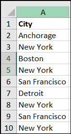
For example, we want to find the count of distinct values in the following list:
To do that use the following formula:
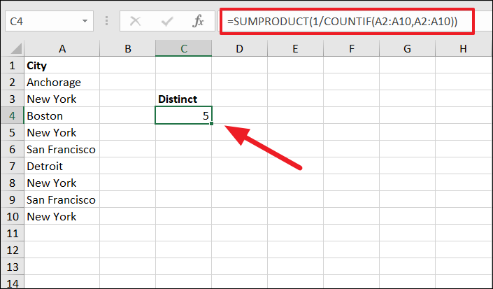
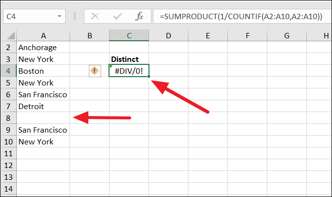
=SUMPRODUCT(1/COUNTIF(A2:A10,A2:A10))Let us break it down for you:
COUNTIF(A2:A10,A2:A10):The nested COUNTIF function counts the number of times each value appears in the cell range (A2:A10) and returns an array of numbers like this:{1;4;1;4;2;1;4;2;4}. i.e. The value that appears only once is 1, the value that appears 4 times is 4, etc.1/COUNTIF(A2:A10,A2:A10): After that, the resulting array of numbers from the COUNTIF formula is used as a divisor/divider for the division with1as their numerator. So 1 is divided by each value of COUNTIF’s array of results. As a result, you will get another array of result:{1;0.25;1;0.25;0.5;1;0.25;0.5;0.25}.
As you can see, the value that appears only once (unique) are 1, and values that appear multiple times will become fractions. For example, the value ‘San Francisco’ appears twice, so when 1 is divided by 2, you will get ‘0.5’.
Finally, the SUMPRODUCT function adds up all numbers in the array and returns the count of distinct values: ‘5’. The count includes all the different values that appear at least once in the list, excluding the duplicates.
Count Distinct Values Ignoring/Including Blank Cells using SUMPRODUCT and COUNTIF Formula
However, when using the above formula if any cell in the range is blank or empty, the formula might throw #DIV/0 error. It’s because a blank cell will produce 0 in the result array created by the COUNTIF formula. So, when 1 is divided by 0, it will result in a #DIV/0 error as shown below.
You can solve this by adding an empty string (“”) as a criterion for the COUNTIF formula.
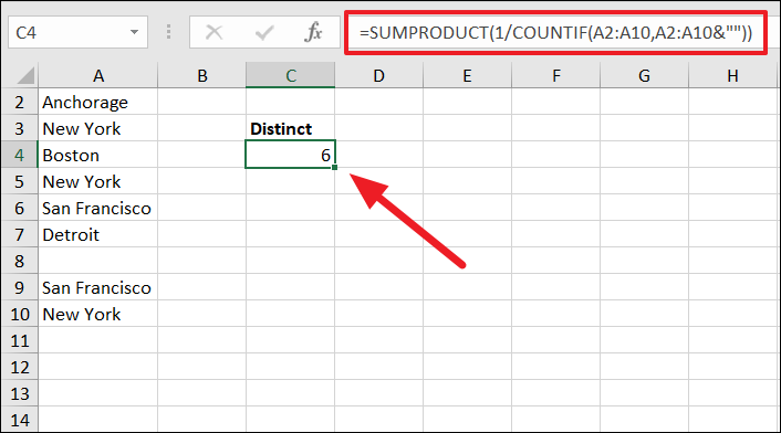
To include blank or empty cells in the count while counting distinct values, try the below formula:
=SUMPRODUCT(1/COUNTIF(A2:A10,A2:A10&""))As you can see above, when we concatenate an empty string (“”) to the data in the criteria argument of COUNTIF function, it returns 1 for an empty cell in the array of results: {1;4;1;4;2;1;1;2;4}. So the formula, 1/COUNTIF(A2:A10,A2:A10&"") = {1;0.25;1;0.25;0.5;1;1;0.5;0.25}. Hence, the final result for distinct values is 6 which also includes the empty cell in the count.
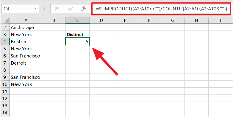
To ignore blank or empty cells from the count while counting distinct values, use the below formula:
=SUMPRODUCT((A2:A10<>"")/COUNTIF(A2:A10,A2:A10&""))Here, A2:A10<>"" produces a TRUE or FALSE array of results. When a cell is empty or blank in the range, it returns FALSE. So when the FALSE value is divided by any number, it returns 0. As a result, now this formula (A2:A10<>””)/COUNTIF(A2:A10,A2:A10&””) returns this array: {1;0.25;1;0.25;0.5;1;0;0.5;0.25}. When summed up, you will get ‘5’ as the final count.
Count Distinct Values using SUM and COUNTIF Functions
Another way you can calculate the number of unique values in Excel is to use the SUM and COUNTIF function together. The SUM and COUNTIF formula works the same as the SUMPRODUCT and COUNTIF functions. The only difference is that is this is an array formula, so it needs to be executed as such by pressing Ctrl+Shift+Enter after typing the formula.
The syntax:
=SUM(1/COUNTIF(range,range))Example:
=SUM(1/COUNTIF(A2:A11,A2:A11))This formula works in a similar way as the SUMPRODUCT method. 1/COUNTIF(A2:A11,A2:A11) returns this array of results {1;0.33;1;0.33;0.5;1;0.5;0.5;0.33;0.5} which are then summed up by the SUM function and shows the distinct values count as 6.
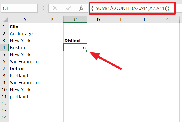
When you press Ctrl+Shift+Enter to execute the formula, the curly brackets will be automatically applied.
Ignore Blank Cells from Distinct Values Count
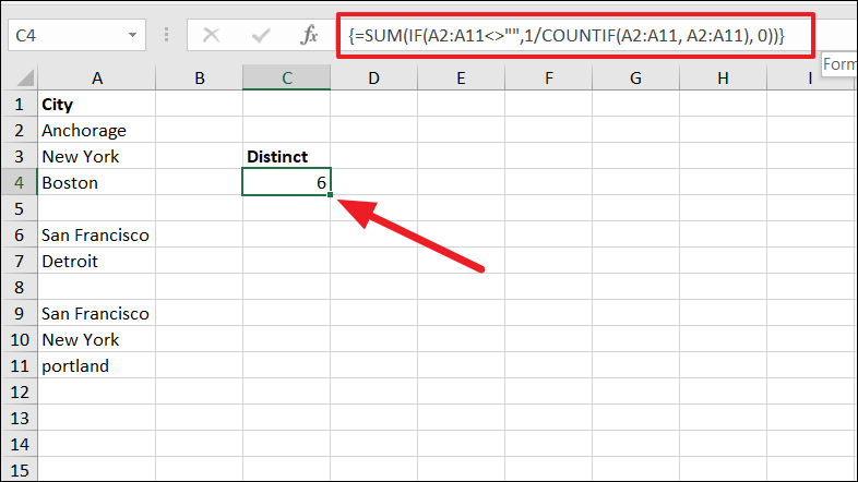
If you wish to ignore blank or empty cells when counting distinct values and avoid #DIV/0! error, you need to enter the following formula:
=SUM(IF(A2:A11<>"",1/COUNTIF(A2:A11, A2:A11), 0))The above formula will ignore the blank cells from the count and returns distinct values count as shown below.
Count Only Distinct Text Values using SUM and COUNTIF Functions
If you have a list of text and number values in a column and you only want to count distinct values that are text values, you have to embed the ISTEXT function into the SUM and COUNTIF formula.
Here is the generic formula for counting distinct text values only:
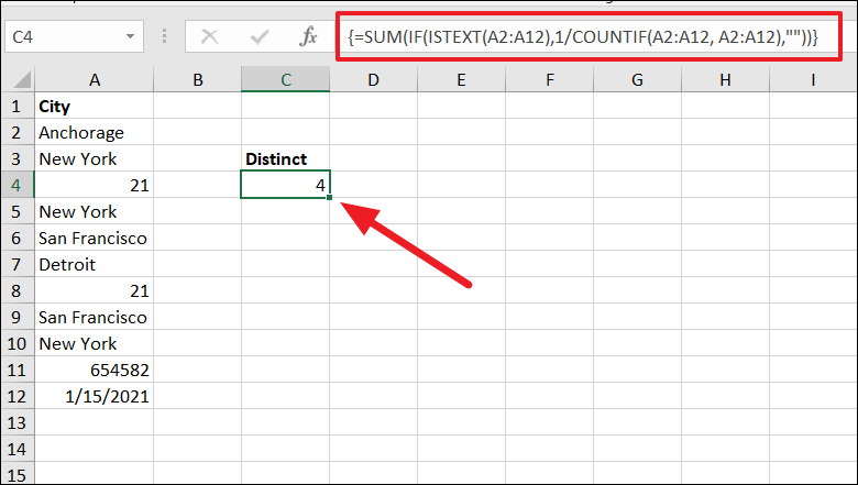
=SUM(IF(ISTEXT(range),1/COUNTIF(range, range),""))For example, we only want to count distinct city names (text values) ignoring number values in the below example. To do that, use the following formula:
=SUM(IF(ISTEXT(A2:A12),1/COUNTIF(A2:A12, A2:A12),""))This is an array formula, so make sure to hit Ctrl+Shift+Enter after writing the formula.
First, the ISTEXT function checks each value in the data range A2:A12 whether it is text or not, and returns TRUE if a value is a text and FALSE for other values. Next, if a value is TRUE, then the IF function tells the COUNTIF function to check and count the number of times that value appears in the given data range (A2:A12). If a value is FALSE, the output will be blank. This will return an array of results: {1;3;””;3;2;1;””;””;2;3;1;1} which are then used as divisors with 1 as the numerator.
Finally, the SUM function adds all the values from the results of 1/COUNTIF(A2:A12, A2:A12) and shows the output as 4 distinct values.
Count Only Distinct Number Values using SUM and COUNTIF Functions
In case you only want to count distinct numbers, dates, and times from a list of values then you can use the generic formula below. This formula is very similar to the above formula except you will be using the ‘ISNUMBER’ function instead of ISTEXT. The Dates and Times are stored as numbers in Excel, so they will also be included in the count.
Syntax:
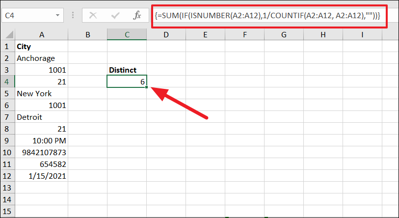
=SUM(IF(ISNUMBER(range),1/COUNTIF(range, range),""))To count distinct numeric values (numbers, dates, and times), write the below formula:
=SUM(IF(ISNUMBER(A2:A12),1/COUNTIF(A2:A12, A2:A12),""))This is an array formula, so make sure to hit Ctrl+Shift+Enter after entering the formula to execute it.
Here, the ISNUMBER checks whether each cell in the range contains a numeric value or not and returns TRUE if a value is a number. If a value is TRUE, the COUNTIF function counts the number of times that number appears in the range. After that, the results from the COUNTIF function are used as the denominator with 1 as the numerator.
At last, the SUM function adds up all the distinct values which are numbers and returns the result.
Count Case-Sensitive Distinct Values using SUM, EXACT, and COUNTIF Functions
If you want to count case-sensitive distinct values, you have to create a helper column with the help of the EXACT function instead of COUNTIF in the array formula to identify the distinct values in a range. Then, a separate COUNTIF formula is used to count those distinct values.
To count case-sensitive distinct values, use the below sample formula:
=IF(SUM((--EXACT($A$2:$A2,$A2)))=1,"Distinct","")Since this is an array formula, you need to press Ctrl+Shift+Enter. After executing the formula, copy it to the rest of the rows using the fill handle. Here’s how this formula works:
The EXACT function checks each value against every value in the range. And if there is no exact value (with the same case characters) is found or if it’s the first instance of the value, it returns ‘Distinct’ otherwise it returns an empty cell.
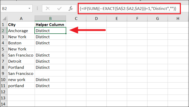
After you got “Distinct” entries in the helper column, you can enter a COUNIF formula to count those entries. To do that enter the below formula in an empty cell:
=COUNTIF(B2:B11,"Distinct")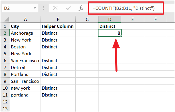
Now, you got the count of case-sensitive distinct values.
Count Distinct Values using SUM, FREQUENCY, and MATCH Functions
The SUM COUNTIF and SUMPRODUCT COUNTIF combos work best if you have small or medium-sized datasets. However, if you have a large dataset, using those combinations can slow down your calculation and may even make your worksheets unresponsive.
So, if you have a large dataset, it is better to use FREQUENCY and MATCH functions to find the count of distinct values. The frequency function returns the number of occurrences for a value in the dataset while the MATCH function returns the relative position of that value in the range. When combined these functions can return the count of distinct values.
Example:
=SUM(IF(FREQUENCY(MATCH(A2:A11,A2:A11,0),MATCH(A2:A11,A2:A11,0))>0,1))This formula does the same thing as the SUM and COUNTIF formula. The only difference is that we are using FREQUENCY and MATCH functions instead. Here, MATCH functions are the two arguments of the FREQUENCY function.
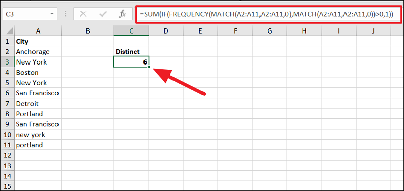
The MATCH function returns the position of each value. Then, the FREQUENCY function check number of occurrence for each value and returns 1 for the first occurrence of the values and 0 for the rest of the occurrences. As a result, the FREQUENCY function creates an array of values. Then each result of the array is checked whether it ‘>0’ and return 1 if it is TRUE. Finally, all those values are summed up by the SUM function to give us the count of distinct values.
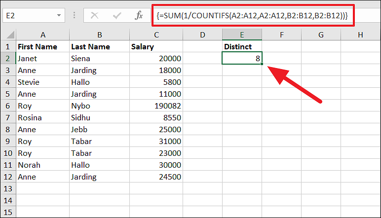
Count Distinct Rows using COUNTIFS function
The above formulas can only help you find the number of distinct values in a single column, but what if you want to count the distinct rows of values across multiple columns? For example, let us say you have a dataset where multiple students have the same first names, and you only want to count distinctive student records (rows) where at least one of the names (either first name or last name) is different.
Counting distinct rows is similar to counting distinct values, the only difference is that you will be using the COUNTIFS function instead of COUNTIF. COUNTIFS function returns the count of cells that meet one or more conditions.
To count distinct rows (students) using the values in column A (First name) and column B (Last name), use the below formula:
=SUM(1/COUNTIFS(A2:A12,A2:A12,B2:B12,B2:B12))Here, COUNTIFS(A2:A12,A2:A12,B2:B12,B2:B12) counts the number of times each row appears across two columns and returns an array of results {1;3;1;3;1;1;1;2;2;1;3} where if at least one of the values in two columns is different, it returns 1. Then, the array of numbers from the COUNTIFS formula is used as a divider with 1 as their numerator. So the array of results from COUNTIFS will become {1;0.33;1;0.33;1;1;1;0.5;0.5;1;0.33}.
Then, the SUM function sums up the array and outputs the result: 8.
Counting Unique Values using Formulas in Excel
You have seen how to calculate distinct values, now let us see how you can find out the number of unique values that appear only once in a list. Just like the count of distinct values, you can get a count of unique values using various Excel function combos.
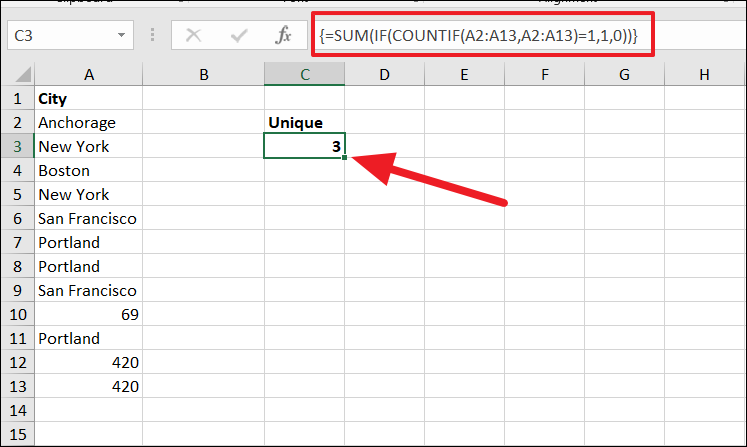
Count Unique Values using SUM, IF, and COUNTIF functions
The easiest way to calculate the count of unique values is to use the SUM function in combination with IF and COUNTIF.
Syntax:
=SUM(IF(COUNTIF(range, range)=1,1,0))Where range is the data range of the list where you want to count the number of unique values.
Example:
Suppose you have a column of cities and you only want to find out the number of cities that only appears only once in the list, then you can use the following formula:
=SUM(IF(COUNTIF(A2:A13,A2:A13)=1,1,0))This is an array formula, so press Ctrl+Shift+Enter to enter the formula.
Here, the nested COUNTIF(A2:A13,A2:A13) function counts the number of times each value appears in cell range (A2:A13) and returns an array of numbers like this: {1;2;1;2;2;3;3;2;1;3;2;2}. The IF function returns 1 if a value in the array of result = 1. If the condition is FALSE, it returns 0. This will turn the array returned by COUNTIF into a different array like this: {1;0;1;0;0;1;0;0;0;0;0;0}. Then, the SUM function adds up the values in the array and gives us the count as ‘3’.
The above formula counts the number of unique values from all kinds of values (text, number, date, etc). But if you only want to count the unique numerical or text values, you will need to use the below formulas.
Count Only Unique Text Values using SUM, COUNTIF, and ISTEXT Functions
If you only want to count the number of unique text values in a list that contains both number and text values, you can use the ISTEXT function along with SUM and COUNTIF functions.
The formula below only counts the unique text values:
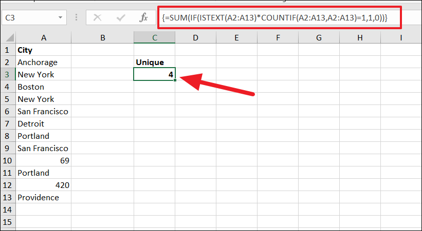
=SUM(IF(ISTEXT(A2:A13)*COUNTIF(A2:A13,A2:A13)=1,1,0))Also, remember to press Ctrl+Shift+Enter to complete it.
- The
COUNTIF(A2:A13,A2:A13)counts the number of times each value appears in the cell range (A2:A13) and returns an array:{1;2;1;2;2;1;2;2;1;2;1;1}. - And the
ISTEXTfunction returns TRUE if a value in the list is TEXT otherwise, it returns FALSE. - Then the AND (*) operator is used to multiply the results of both arguments. If a number (any number) is multiplied by FALSE, it will return 0 and if a number is multiplied by TRUE will return the same number. ( e.g. 1*TRUE=1, 2*FALSE=0, 2*TRUE=2)
- As a result, the IF function will return 1 if a value is both text (TRUE) and unique (1) i.e. if TRUE*1=1, the function returns 1, otherwise 0. This will create an array:
{1;0;1;0;0;1;0;0;0;0;0;1)where 1 is a text and unique value.
At last, the SUM function sums up the values in the array returned by IF and shows the number of unique text values in the column: 4.
Count Unique Numeric Values using SUM, COUNTIF, and ISNUMBER Functions
To count only numerical values in a list, add the ISNUMBER function instead of ISTEXT to the array formula (Ctrl+Shift+Enter):
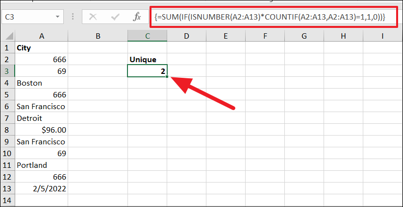
=SUM(IF(ISNUMBER(A2:A13)*COUNTIF(A2:A13,A2:A13)=1,1,0))The ISNUMBER function returns TRUE if a value in the list is a number otherwise, it returns FALSE. The COUNTIF(A2:A13,A2:A13) counts the number of times each value appears in the cell range (A2:A13) and returns this array : {3;2;1;3;2;1;1;2;2;1;3;1}.
When the results of both functions are multiplied, the IF function returns 1 only if a value is both number and unique, 0 otherwise. Finally, the SUM function adds up the values returned by the IF function and gives the number of unique numbers: 2.
Count Case-Sensitive Unique Values in Excel
In case you want to count case-sensitive unique values, you have to create a helper column with the help of the EXACT function instead of COUNTIF in the array formula to identify the unique values in the range. Then, you can use the COUNTIF formula to count those unique values from the helper column.
You can use the following array formula to count case-sensitive unique values:
=IF(SUM((--EXACT($A$2:$A$12,A2)))=1,"Unique","Duplicate")Complete the formula by hitting Ctrl+Shift+Enter together. After that, drag the fill handle to apply the formula to the rest of the column.
In the above formula, the EXACT function checks each value against every value in the range. And if there is no exact value (with the same case characters) is found, it returns ‘Unique’ otherwise it returns ‘Duplicate’.
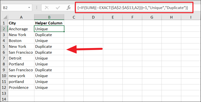
The above formula returns ‘Unique’ in the Helper Column if the corresponding value is case-sensitive unique otherwise, it returns ‘Duplicate’. As you can see both “new york” and “portland” values already appear in the list, however, these values are in different cases. So, they returned as ‘Unique’ in the helper column.
Then, you can enter a COUNIF formula to count those entries. To do that enter the below formula in an empty cell:
=COUNTIF(B2:B12,"Unique")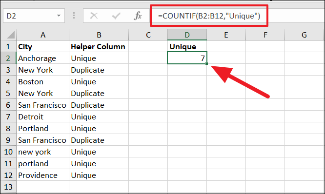
Now, you got the number of case-sensitive unique values in cell D2.
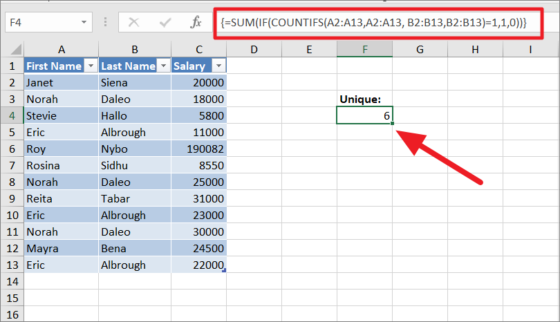
Count Unique Rows using COUNTIFS function
Counting unique rows is similar to counting unique values, the only difference is that you will be using the COUNTIFS function instead of COUNTIF.
If you wish to count unique rows (students) using the values in column A (First name) and column B (Last name), use the below formula:
=SUM(IF(COUNTIFS(A2:A12,A2:A12,B2:B12,B2:B12)=1,1,0))Here, COUNTIFS(A2:A12,A2:A12,B2:B12,B2:B12) counts the number of times each row appears in the list and returns an array of results {1;3;1;3;1;1;1;2;2;1;3} where if at least one of the values (First name or Last name) in two columns is unique, it returns 1. Then, if a value from the COUNTIFS array is equal to 1, the IF function returns 1, 0 otherwise. As a result, the COUNTIFS array becomes {1;0;1;0;1;1;1;0;0;1;0}. Finally, the SUM function adds up the array and outputs the result as 6.
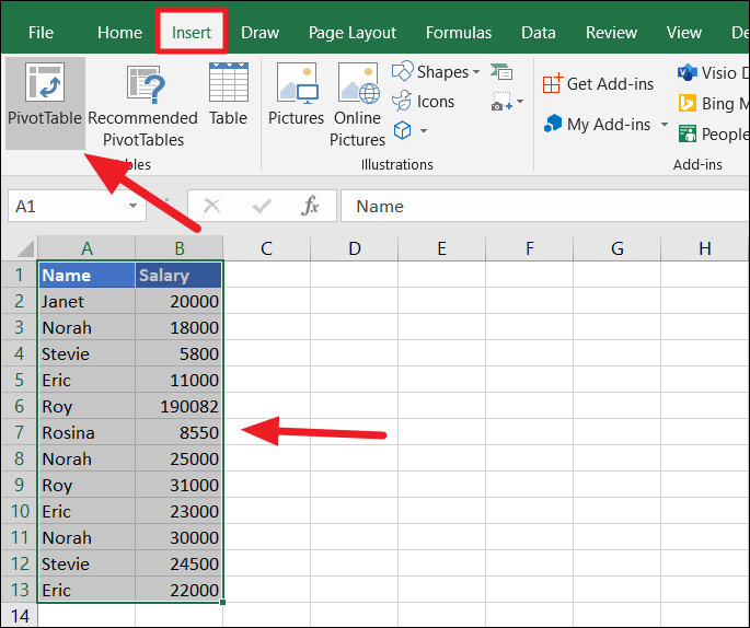
Count Distinct Values using Pivot Table
If you are using Excel 2013 or a later version (including Office 365), you can count distinct values using a pivot table. To count the distinct values using a pivot table, follow these steps:
To start with, select the range of cells you want to be included in a pivot table, then go to the ‘Insert’ tab and click ‘Pivot Table’ from the Tables group.
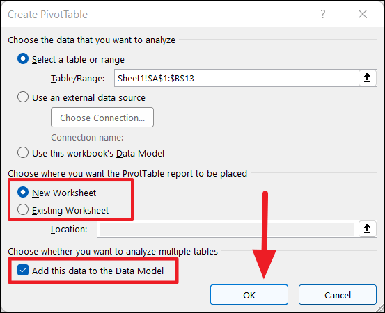
When the Create PivotTable dialog appears, choose whether you want to place your pivot table in a ‘New Worksheet’ or ‘Existing Worksheet’. Then, check the ‘Add this data to the Data Model’ box and click ‘OK’. If you choose to place the pivot table in the current worksheet, specify a range in the location field. Here, we’re selecting a new worksheet.
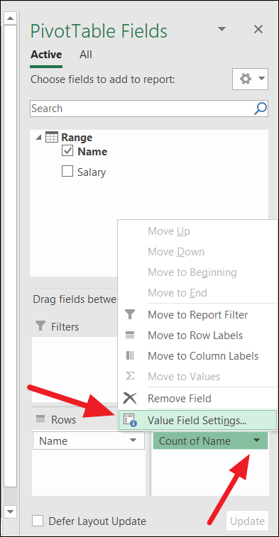
You will see the PivotTable fields pane on the right side of the worksheet. Now, drag the field (column) whose distinct count you want to find to the ‘Values’ area. Here, we want to find distinct values for the ‘Name’ field. You can arrange your data in the pivot table fields in any way you want.
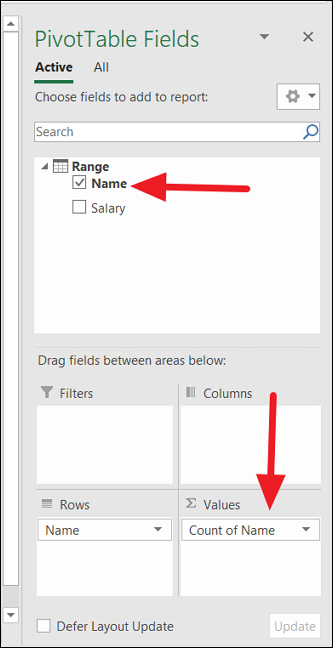
Next, click on the small arrow next to ‘Count of Name’ in the Values field in the Pivot Table fields pane and select the ‘Value Field Settings..’ option.
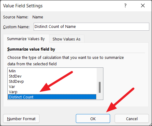
In the Value Field Settings dialog box, scroll down the list in the box and select the ‘Distinct Count’ option at the end of the list. Then, click ‘OK’.
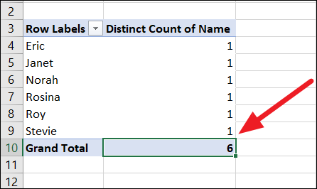
This will show the count of unique values in the pivot table as shown below.
Count Unique Values using User Defined Function (UDF)
Another way can calculate unique values is to create your User Defined Function (UDF) and use that function to count unique values in your list. To do that follow these steps:
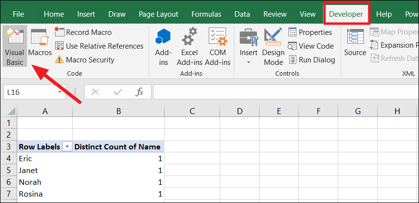
First, open Excel, go to the ‘Developer’ tab and click the ‘Visual Basic’ button in the Code group.
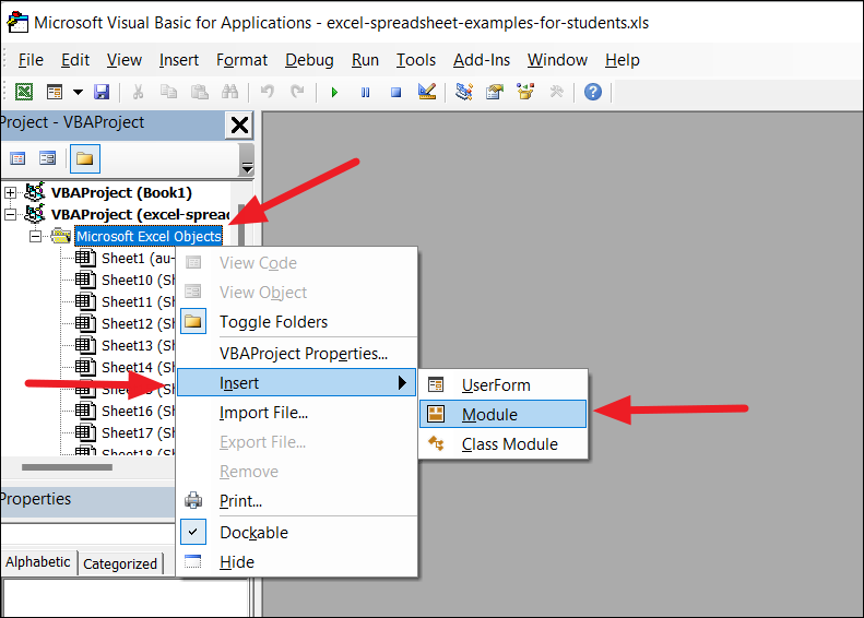
This will launch the VBA window. Now, right-click on the ‘Microsoft Excel Objects’ in the navigation bar on the left, click ‘Insert’, and then ‘Module’ in the sub-menu (as shown below).
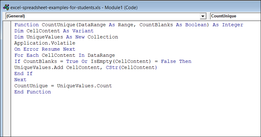
In the new module window, copy and paste the following UDF code:
Function CountUnique(DataRange As Range, CountBlanks As Boolean) As Integer
Dim CellContent As Variant
Dim UniqueValues As New Collection
Application.Volatile
On Error Resume Next
For Each CellContent In DataRange
If CountBlanks = True Or IsEmpty(CellContent) = False Then
UniqueValues.Add CellContent, CStr(CellContent)
End If
Next
CountUnique = UniqueValues.Count
End Function
In the above UDF code, we used the function name as CountUnique. But you can use any name you want for your function.
Then, click the ‘File’ menu and select ‘Save’ or simply press Ctrl+S.
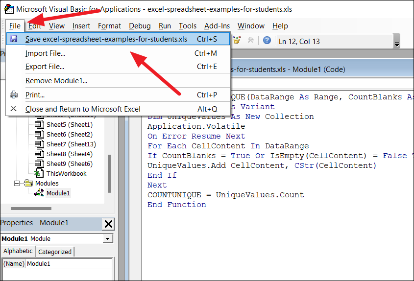
You have created your own new function called CountUnique.
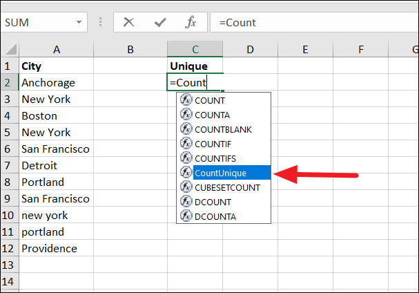
Use UDF to Count Unique Values
Now, you can use the newly created ‘CountUnique’ function (UDF) to count unique values. As you can see, when you start typing the UDF name, you will see it in the formula suggestions as shown below.
To count unique values using UDF, use the below generic formula:
=COUNTUNIQUE(range, count_blanks)Where
rangeis the range of cells (column) where you want to calculate the count of unique values.count_blanksspecifies whether you want to include blank cells in the count or not. You can set TRUE or FALSE for this argument. TRUE if you want to include blank cells in the count, FALSE otherwise.
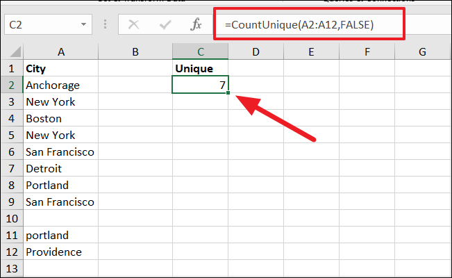
Example formula:
=CountUnique(A2:A12,FALSE)The above formula checks if a value is unique in the range A2:A12 and includes it in the count. The FALSE argument tells the formula not to include any empty cells in the count. If you wish to include the empty cells in the count, set the second argument of the function as TRUE.
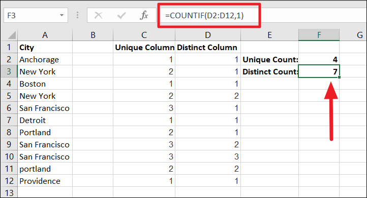
Count Unique and Distinct Values using Helper Columns with COUNTIF function
You can also count both unique and distinct values by building helper columns using the COUNTIF function. Then use another COUNTIF function to count the values in the entries in the builder column. This is one of the easiest ways to count unique and distinct values.
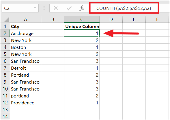
For unique values, create a helper column and enter this formula in cell C2:
=COUNTIF($A$2:$A$12,A2)Then drag the fill handle to copy the formula to the rest of the cells. Here, the range $A$2:$A$12 is made obsolete, so it doesn’t change when copied. Make sure to make only the range is absolute.
After applying the formula to the whole column (C2:C12), it checks each value against every value in the column and returns the number of times each value appears in the column.
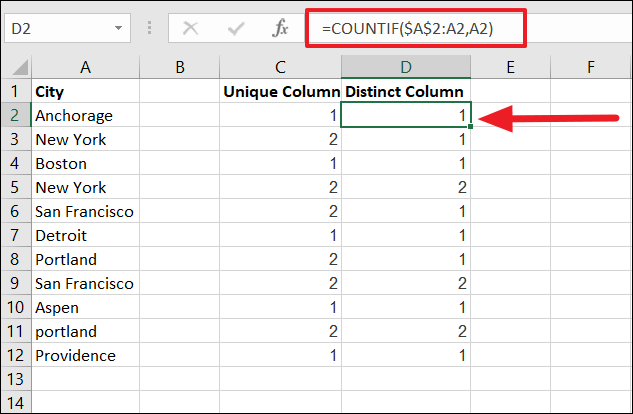
For distinct values, create a helper column and enter this formula in cell D2:
=COUNTIF($A$2:A2,A2)Here, make sure to write only 1st cell of a range absolute. After entering the formula in cell D2, copy the formula to column D2:D12 by dragging the fill handle.
The above formula returns occurrences of the value in the range. For example, the formula in cell D2 checks how many times the value in A2 repeats until cell A12 and returns the occurrence. The formula in cell D5 checks how many times the value in A5 repeats from A2 to A5 and returns its occurrence ( 2 times), and so on. As a result, the formula returns 1 for only the first occurrence of the value.
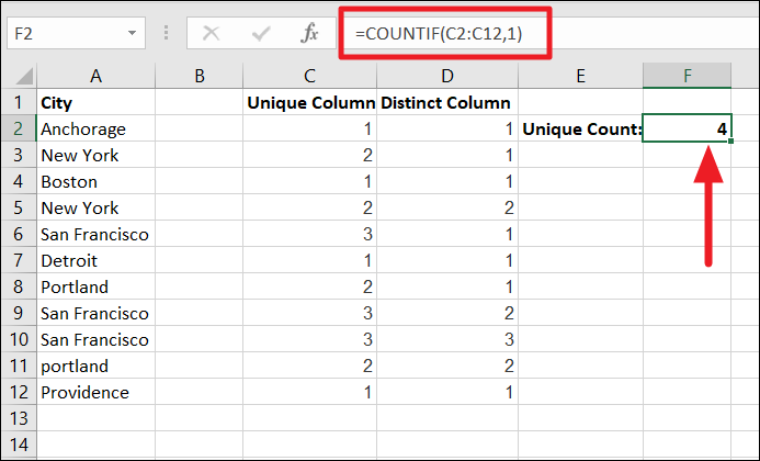
To count unique values, enter this formula:
=COUNTIF(C2:C12,1)Here, the range is C2:C12 and the criterion is 1. The above formula checks the range C2:C12 for the value 1 and if the condition is TRUE, it returns 1, 0 otherwise :{1,0;1;0;0;1;0;0;1;0;1}. Then the array is added up and outputted as the count of unique values: 4.
To count distinct values, enter this formula:
=COUNTIF(D2:D12,1)Here, the range is D2:D12 and the criterion is 1. The formula checks for the values 1 and counts them. As a result, you will get the count of distinct values.
That’s it.


