
Understanding the Compound Annual Growth Rate (CAGR) is crucial for analyzing the performance of investments over time. It represents the smoothed annual growth rate, eliminating the effects of volatility in periodic returns.
Calculating the Compound Annual Growth Rate (CAGR) in Excel
To calculate the CAGR in Excel, you need three essential pieces of information: the beginning value of the investment, the ending value, and the number of periods (typically years). The CAGR formula allows you to determine the mean annual growth rate of an investment, which is particularly useful for comparing different investments over the same time frame.
The formula for calculating CAGR is:
CAGR = (Ending Value / Beginning Value)^(1 / n) - 1
Where:
Ending Value – The final value of the investment at the end of the period.
Beginning Value – The initial value of the investment at the start of the period.
n – The number of periods (years) over which the investment has grown.
Methods to Calculate CAGR in Excel
While Excel doesn’t provide a dedicated CAGR function, there are several methods you can use to compute it:
– Using the RRI function.
– Using the arithmetic formula with operators.
– Using the POWER function.
– Using the RATE function.
– Using the IRR function.
Calculating CAGR in Excel Using the RRI Function
The most straightforward method to calculate CAGR in Excel is by using the RRI function. The RRI function computes the equivalent interest rate for the growth of an investment over a specified number of periods.
The syntax of the RRI function is:
=RRI(nper, pv, fv)Where:
nper – The total number of periods.
pv – The present value (beginning value) of the investment.
fv – The future value (ending value) of the investment.
Suppose we have the revenue data for a company over several years:
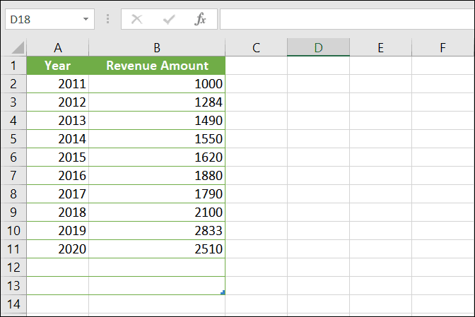
In this dataset, column A lists the years, and column B contains the corresponding revenue figures. To calculate the CAGR using the RRI function:
=RRI(9, B2, B11)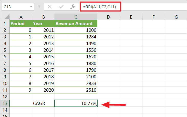
The result will display the CAGR as a decimal. To format it as a percentage, select the cell, navigate to the Home tab, and choose the Percentage option in the Number group.
The calculated CAGR, in this case, is 10.77%, indicating the company’s revenue grew at an average rate of 10.77% per year over the nine-year period.
Calculating CAGR in Excel Using the Arithmetic Formula
You can also calculate the CAGR directly using arithmetic operators by applying the CAGR formula.
=(B11 / B2)^(1 / 9) - 1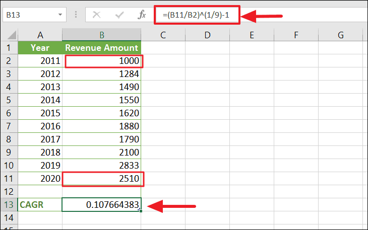
This method provides the same result, a CAGR of 10.77%.
Calculating CAGR in Excel Using the POWER Function
The POWER function can simplify the calculation by replacing the exponentiation operation in the CAGR formula.
The syntax of the POWER function is:
=POWER(number, power)Where:
number – The base number (ending value divided by beginning value).
power – The exponent (1 divided by the number of periods).
=POWER(B11 / B2, 1 / 9) - 1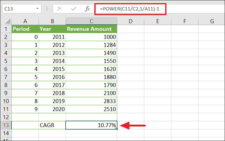
This method also yields a CAGR of 10.77%.
Calculating CAGR in Excel Using the RATE Function
The RATE function calculates the interest rate per period of an annuity. It can be adapted to determine the CAGR.
The syntax of the RATE function is:
=RATE(nper, pmt, pv, [fv], [type], [guess])For calculating CAGR, you can simplify the function by leaving out unnecessary arguments:
=RATE(nper, , -pv, fv)=RATE(9, , -B2, B11)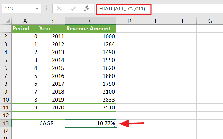
Again, you will arrive at a CAGR of 10.77%.
Calculating CAGR in Excel Using the IRR Function
The IRR function calculates the internal rate of return for a series of cash flows, which can be used to find the CAGR when adjusted appropriately.
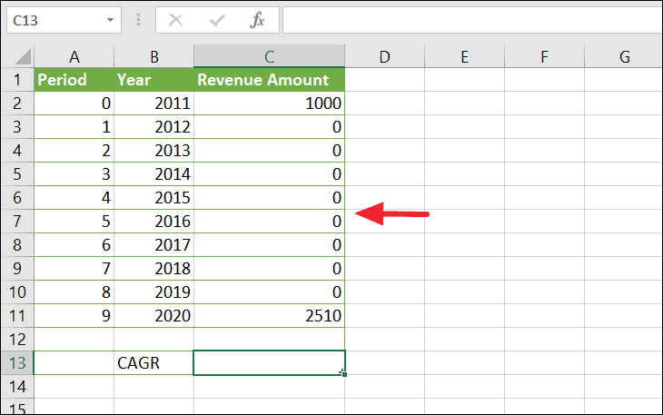
=IRR(B2:B11)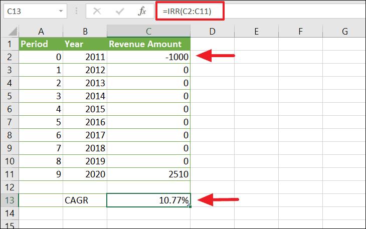
The result will show the CAGR as a percentage.
Calculating the CAGR in Excel is straightforward using these methods. Whether you prefer using built-in functions like RRI or applying the arithmetic formula directly, Excel provides versatile tools to analyze investment growth over time.


