How to Create a Drop Down List in Excel

Drop-down lists in Excel streamline data entry by providing users with predefined options to choose from, reducing errors and saving time.

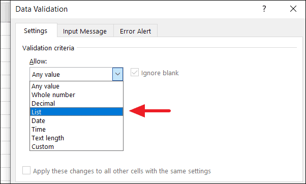
Creating a drop-down list using data from cells

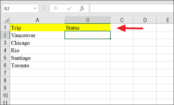
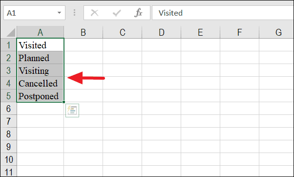
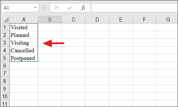
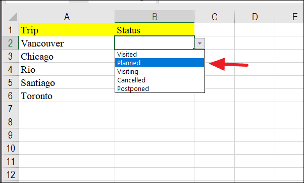
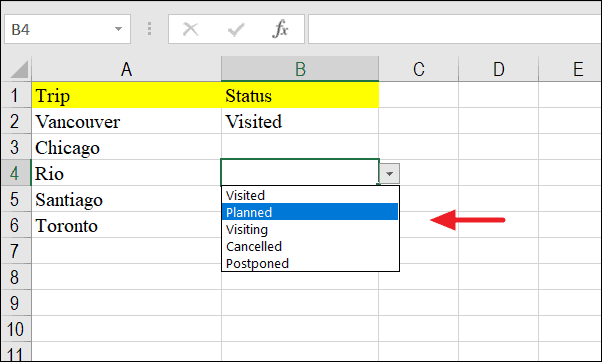
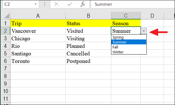
Suppose you’re planning various trips and want to track the status of each one using a drop-down menu. This allows for consistent status updates like “Finished” or “Pending” without manually typing them each time.

Enter the list of statuses you want to include in your drop-down menu into a column of cells. You can do this either in the same worksheet where you want the drop-down or in a different one. In this example, the list is entered in Sheet2.

Go back to Sheet1 and select the cell where you want to place the drop-down menu, such as cell B2 under the “Status” column.

Navigate to the “Data” tab on the Ribbon and click on “Data Validation” in the “Data Tools” group. From the dropdown, select “Data Validation.”

In the “Data Validation” dialog box, under the “Settings” tab, select “List” from the “Allow” dropdown menu.

Click inside the “Source” box, then navigate to the sheet where your list is located (Sheet2) and select the range of cells containing your list (e.g., A1:A5).

The selected range will appear in the “Source” field. Ensure that “Ignore blank” is unchecked if you want to prevent users from leaving the cell empty. Click “OK” to finalize the drop-down list.

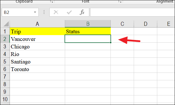
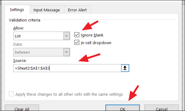
Now, the drop-down list is created in cell B2.

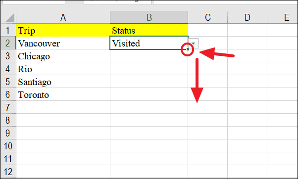
To apply the drop-down list to other cells, select cell B2, then drag the fill handle (the small square at the bottom-right corner of the cell) down to the desired range, such as B2 to B6.

The drop-down list is now copied to the selected cells.

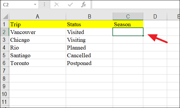
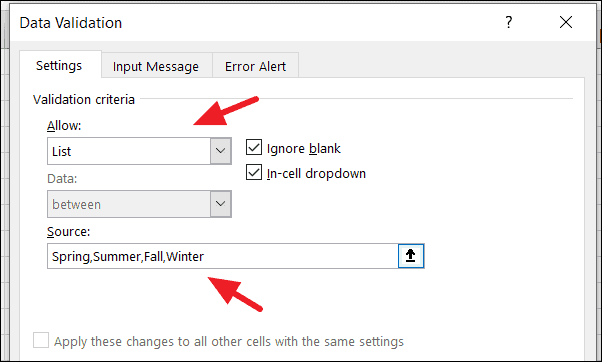
Creating a drop-down list by entering data manually

Alternatively, you can create a drop-down list by typing the items directly into the “Source” field of the Data Validation dialog box. This is useful when you have a small list of items that won’t change.

Select the cell where you want to create the drop-down list, such as cell C2 for the “Season” column.

Go to the “Data” tab and click on “Data Validation” in the “Data Tools” group.

In the Data Validation dialog box, select “List” from the “Allow” dropdown. In the “Source” field, type the items you want in your list, separated by commas without spaces. For example, enter “Spring,Summer,Fall,Winter” and click “OK.”

Now, the items you entered will appear as options in the drop-down list. You can then copy this drop-down to other cells just like before.

Creating a drop-down list using formulas

You can also create a dynamic drop-down list using a formula in the “Source” field. This method allows for more flexibility, especially when dealing with ranges that might change.

Enter the list of items for your drop-down in a column in your worksheet or a different sheet. For example, list the years in cells B1:B5 on Sheet2.

Go back to the sheet where you want the drop-down list and select the cell, such as D1.

Open the Data Validation dialog box from the “Data” tab.

In the “Source” field, enter the OFFSET formula to define the range dynamically. For example:

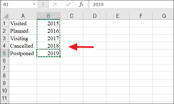
=OFFSET(Sheet2!$B$1,0,0,5)

This formula starts at cell B1 on Sheet2 and includes five rows in the range. Adjust the number ‘5’ to match the number of items in your list.

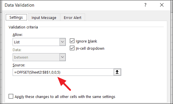
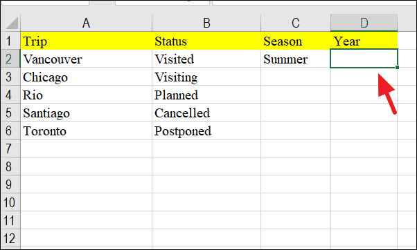
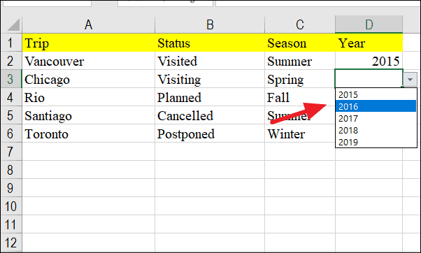
Click “OK” to apply the data validation with the formula. The drop-down list will now display the years from your specified range.

Removing a drop-down list

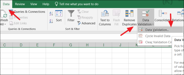
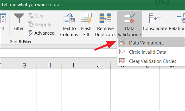
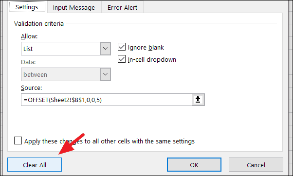
If you need to remove a drop-down list, select the cell containing it. Go to the “Data” tab, click on “Data Validation,” and then click “Clear All” in the dialog box. This will remove the drop-down from the selected cell.

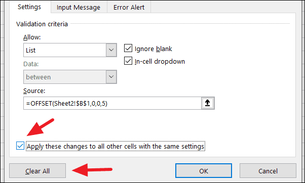
To remove drop-down lists from multiple cells at once, select the cells before opening the Data Validation dialog. Alternatively, check the “Apply these changes to all other cells with the same settings” option before clicking “Clear All,” then click “OK.”

By following these methods, you can efficiently create, apply, and manage drop-down lists in Excel to enhance data entry and maintain consistency across your spreadsheets.