Dividing numbers in Excel is a fundamental task that's essential for various calculations and data analysis. Whether you're working with individual cells, entire columns, or need to use specific functions, Excel provides multiple ways to perform division operations efficiently.
Divide Numbers Using the Forward Slash Operator
The simplest way to divide in Excel is by using the forward slash (/) operator. This method allows you to perform division directly within a cell using basic formulas.
To divide two numbers within a cell, click on an empty cell and type the equals sign (=) to start a formula. Then, enter the dividend (the number to be divided), followed by the forward slash, and then the divisor (the number you are dividing by). The formula looks like this:
=dividend/divisorFor instance, if you want to divide 23 by 4, you would input the following formula:
=23/4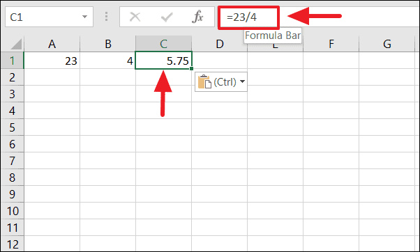
Divide One Cell by Another Cell
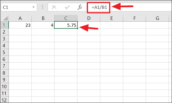
Often, you'll need to divide the value of one cell by another cell. To do this, start by selecting the cell where you want the result to appear. Type the equals sign (=) to initiate a formula, then enter the cell reference of the dividend, followed by the forward slash, and then the cell reference of the divisor. Here's the format:
=Cell1/Cell2For example, to divide the value in cell A1 by the value in cell B1, you would type:
=A1/B1Press Enter, and Excel will display the result in the selected cell.
Divide Entire Columns of Cells
If you have two columns of numbers that you need to divide row by row, you can apply the division formula to an entire range. Begin by entering the division formula in the first cell of your result column. Using our previous example, in cell C1, input:
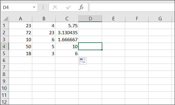
=A1/B1After calculating the first result, you can quickly apply the same formula to the rest of the rows. Click on the cell with the formula (C1), and hover over the small green square at the bottom-right corner of the cell (known as the fill handle). Click and drag the fill handle down to cover all the rows you wish to calculate (e.g., down to cell C5).
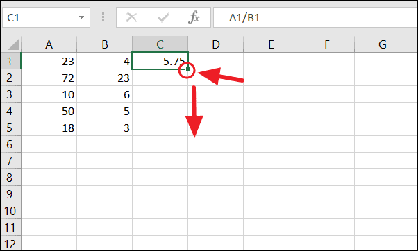
Excel will automatically adjust the cell references for each row, dividing each corresponding pair of cells from columns A and B, and displaying the results in column C.
You can also create more complex division formulas involving multiple cells. For example, to divide the value in A1 by B2, and then divide that result by B1, you would use:
=A1/B2/B1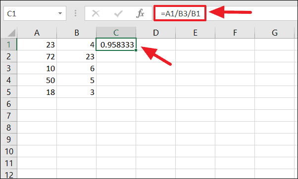
Divide a Range of Cells by a Constant Number
Sometimes, you may need to divide a range of cells by a single constant number. To do this without altering your original data, you can use absolute cell references to lock the divisor in your formula. An absolute reference is created by adding a dollar sign ($) before the column letter and row number of the cell reference.
For example, if you have numbers in cells A1 through A5 and you want to divide each by the constant number in cell A7, you would proceed as follows:
In cell C1, enter the formula:
=A1/$A$7The $A$7 reference ensures that when you copy the formula down, the divisor remains the constant value in cell A7.
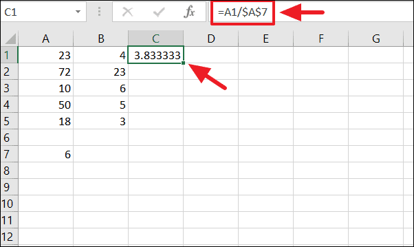
After entering the formula in cell C1, use the fill handle to drag the formula down from C1 to C5. Each cell in column C will now contain the result of dividing the corresponding value in column A by the constant value in A7.
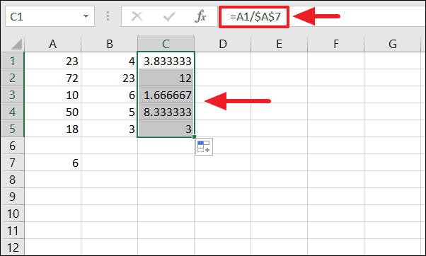
Divide a Column by a Constant Number Using Paste Special
An alternative method to divide a range of cells by a constant number is by using the Paste Special feature. This method overwrites the original values with the results of the division.
Step 1: Copy the cell containing the constant number. Right-click on cell A7 and select Copy or press Ctrl + C.
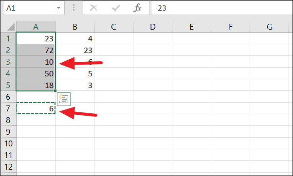
Step 2: Select the range of cells you want to divide (e.g., A1:A5). Right-click within the selected range and choose Paste Special.
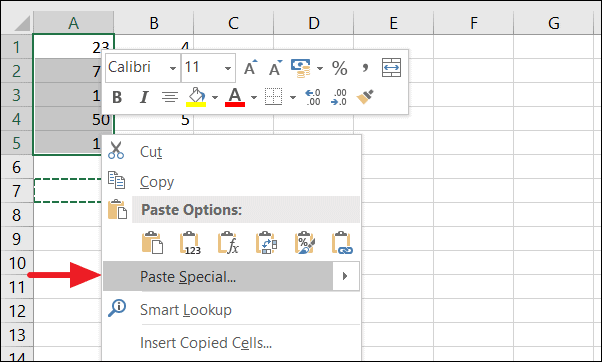
Step 3: In the Paste Special dialog box, under the Operation section, select Divide. Click OK to apply the operation.
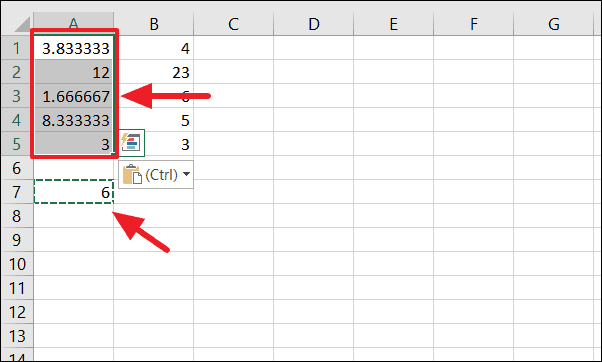
This action will divide each cell in the selected range by the constant number in cell A7. Note that this method replaces the original values in A1:A5 with the division results, so you may want to copy the original data to another location if you need to preserve it.
Divide Using the QUOTIENT Function
Excel's QUOTIENT function allows you to perform division operations that return only the integer portion of the result, discarding any remainder. This can be useful when you need to know how many times a number can be divided by another number completely.
The syntax for the QUOTIENT function is:
=QUOTIENT(numerator, denominator)For example, to divide 50 by 5 using the QUOTIENT function, you would use:
=QUOTIENT(50, 5)This returns 10, which is the same as using the division operator since 50 divided by 5 leaves no remainder.
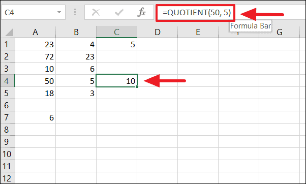
However, when there's a remainder, the QUOTIENT function will not include it in the result. For instance, dividing 23 by 4 using QUOTIENT(23, 4) will return 5, whereas using the division operator =23/4 returns 5.75.
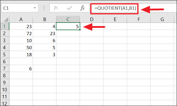
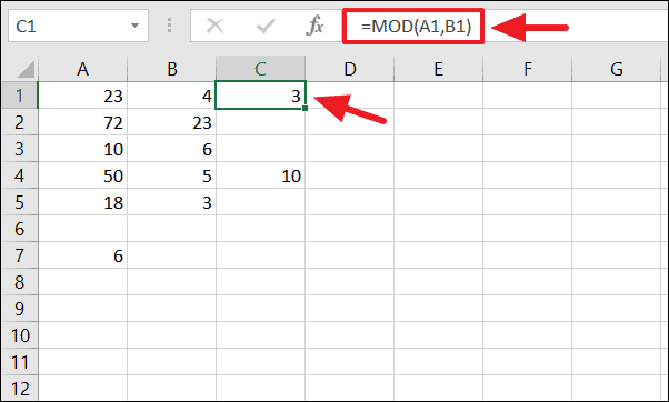
If you're interested only in the remainder of a division operation, you can use the MOD function. For example:
=MOD(23, 4)This formula returns 3, which is the remainder when 23 is divided by 4.
#DIV/0! Error and How to Avoid It
While performing division in Excel, you might encounter the #DIV/0! error. This error occurs when a number is divided by zero or when a formula refers to a blank cell or a cell containing zero as the divisor. Since division by zero is undefined, Excel cannot compute the result.
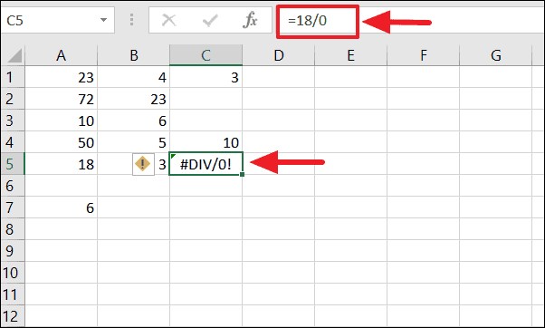
To prevent this error, ensure that your divisor is not zero or adjust your formulas to handle such cases. You can use the IFERROR function to display a custom message or an alternate result when an error occurs. For example:
=IFERROR(A1/B1, "Division by zero")Mastering division in Excel enhances your ability to handle data effectively. Whether you're using simple operators or leveraging built-in functions, these methods will help you perform division tasks with confidence.

