Circular references in Excel arise when a formula refers back to its own cell, either directly or indirectly, leading to endless loops and potential calculation errors. This happens when a formula needs the result of its own cell to compute, causing Excel to repeatedly recalculate without reaching a conclusion.
For instance, imagine cells B1 and B2 contain numbers. If you enter the formula =B1+B2 into cell B2, the formula in B2 now includes itself in the calculation, creating a circular reference. Each time Excel tries to compute the value of B2, it changes, triggering another recalculation.
While most circular references are unintended mistakes, some are deliberate, used for iterative calculations. Unintended circular references can cause formulas to produce incorrect results or slow down your worksheet. Therefore, it’s crucial to understand how to find, handle, and resolve circular references in Excel.
Identifying and Managing Circular References
Circular reference errors occur when a formula in a cell refers back to itself. This can cause calculators to loop indefinitely, which Excel detects and warns you about. Knowing how to find and fix these errors ensures your data remains accurate.
Consider a scenario where you have numbers in cells A1 through A4 and you use the SUM function in cell A5 with the formula =SUM(A1:A5). Here, A5 is included in the range of the SUM function that’s placed in A5 itself, creating a direct circular reference. Excel will display a warning message indicating a circular reference has been detected.
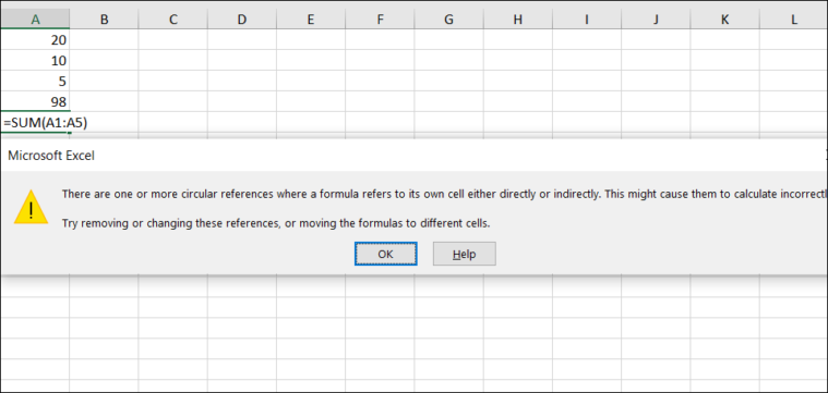
After this warning appears, you can click ‘Help’ to learn more about the error or ‘OK’ to dismiss it. The result of the formula will typically display as zero. Circular references can lead to miscalculations and may slow down your worksheet’s performance, so it’s important to resolve them promptly.
Types of Circular References
Circular references in Excel can be categorized into two types: direct and indirect.
Direct Circular References
A direct circular reference occurs when a formula refers directly to its own cell. For example, if you enter the formula =A2+1 into cell A2, the formula is directly dependent on its own cell, prompting Excel to display a circular reference warning.
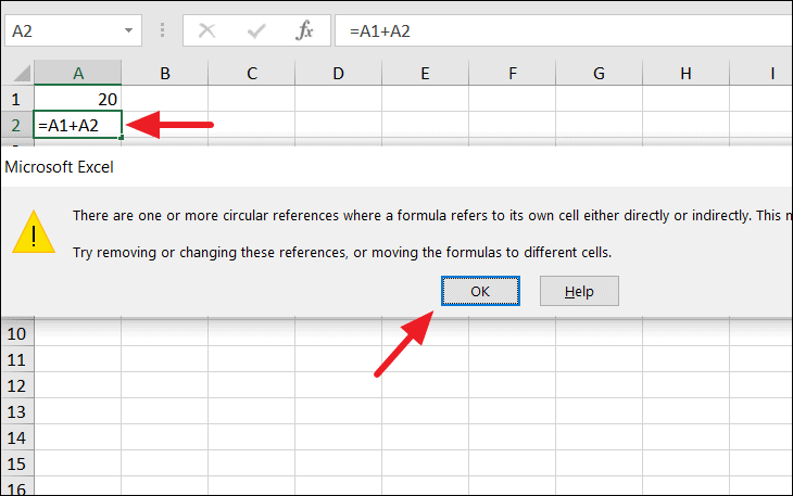
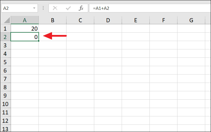
When the warning appears, clicking ‘OK’ will result in the cell displaying zero, as Excel cannot compute a value due to the circular dependency.
Indirect Circular References
An indirect circular reference happens when a formula refers to another cell that eventually refers back to the original cell. This creates a loop of dependencies that is not immediately obvious.
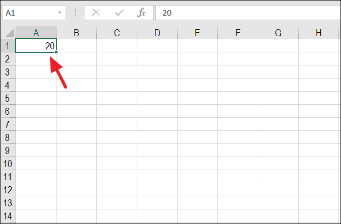
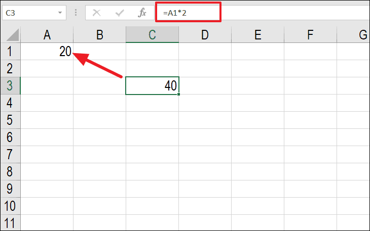
For example, suppose cell A1 contains a value of 20.
Cell C3 contains the formula =A1.
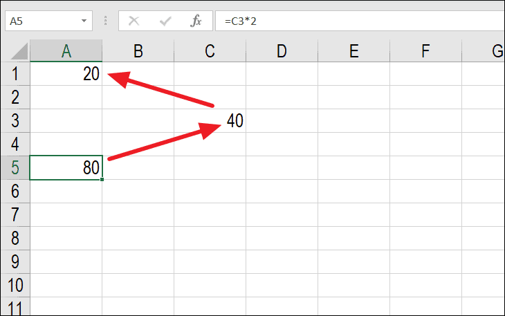
Cell A5 refers to cell C3 with the formula =C3+5.
Now, if you replace the value in cell A1 with a formula that refers to A5, like =A5*2, a circular reference is created because A1 depends on A5, which in turn depends on C3, which refers back to A1.
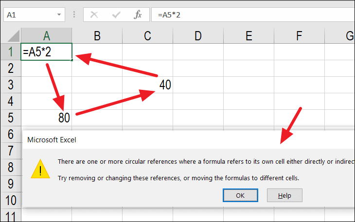
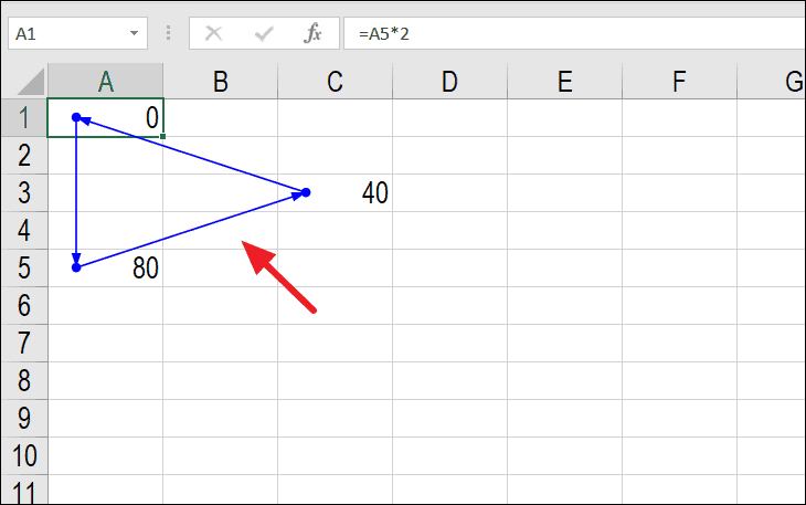
Clicking ‘OK’ on the warning will result in the cell showing zero, and Excel may display tracer arrows indicating the circular relationship. These visual cues can help identify and resolve circular references.
Enabling or Disabling Circular References
By default, Excel disables iterative calculations, which prevents formulas from repeatedly recalculating. When iterative calculations are off, Excel alerts you to any circular references and returns zero as the result. However, in certain cases, you might need to enable iterative calculations to allow intentional circular references for iterative computations.
To enable iterative calculations:
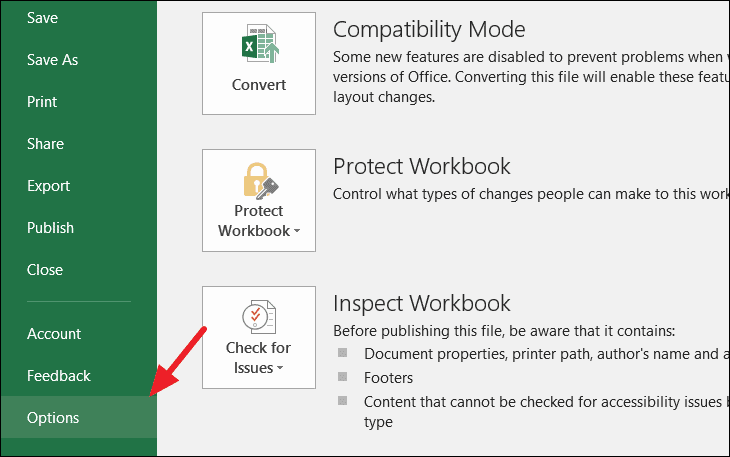
In Excel 2010 and later versions, navigate to the ‘File’ tab and select ‘Options’.
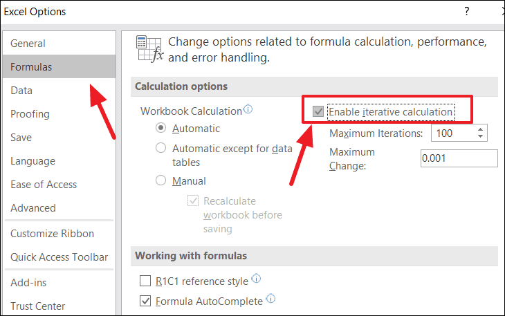
In the Excel Options window, choose ‘Formulas’ from the sidebar. Under the ‘Calculation options’ section, check the box labeled ‘Enable iterative calculation’. Click ‘OK’ to apply the changes.
For earlier versions of Excel:
- In Excel 2007, click the Office button, then select ‘Excel Options’ > ‘Formulas’ > check ‘Enable iterative calculation’.
- In Excel 2003 and earlier, go to the ‘Tools’ menu, select ‘Options’, and then the ‘Calculation’ tab to enable iterative calculations.
Adjusting Iterative Calculation Settings
When enabling iterative calculations, you can specify the ‘Maximum Iterations’ and ‘Maximum Change’ parameters to control how Excel handles calculations.
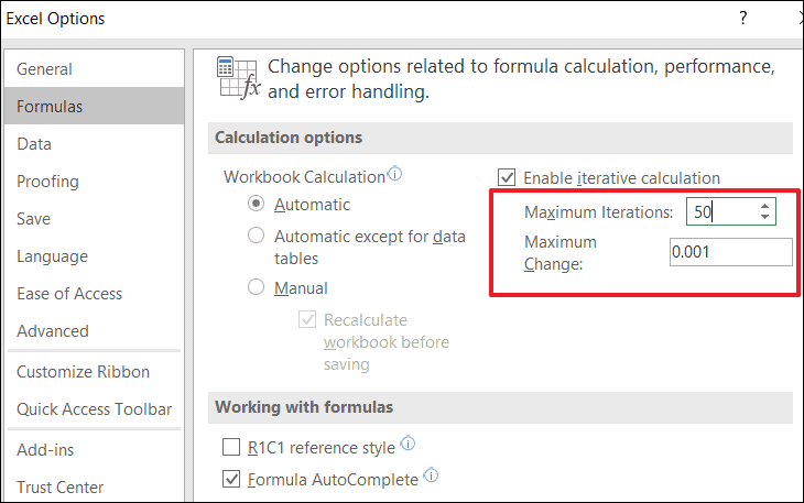
- Maximum Iterations: Sets the number of times Excel recalculates. A higher number means more attempts to reach a solution but can slow down performance.
- Maximum Change: Defines the smallest change between calculation results. Smaller numbers increase accuracy but may require more iterations.
Only enable iterative calculations when necessary, as turning it on will prevent Excel from warning you about circular references.
Locating Circular References
When dealing with large worksheets, finding the exact location of a circular reference can be challenging. Excel provides tools to help identify these cells so you can address the issue.
Using the Error Checking Tool
Open the worksheet where the circular reference is present. Go to the ‘Formulas’ tab, click the small arrow next to ‘Error Checking’, and hover over ‘Circular References’. A list of cells involved in circular references will appear.
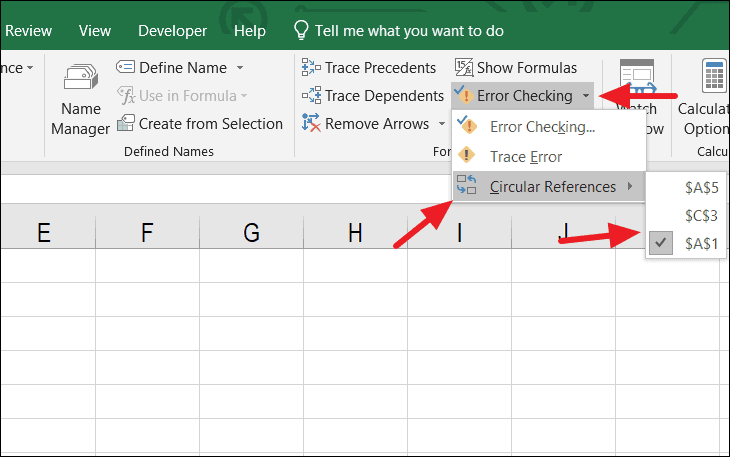
Select a cell from the list to navigate directly to it and resolve the circular reference.
Using the Status Bar
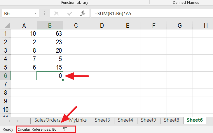
The status bar at the bottom of Excel can also alert you to circular references. It will display ‘Circular References’ followed by the cell address of the most recent circular reference detected, such as ‘Circular References: B6’.
Keep in mind:
- The status bar will not show circular references if iterative calculations are enabled.
- If the circular reference is on a different sheet, the status bar will display ‘Circular References’ without a cell address.
- The warning prompt appears only once per session unless you resolve the circular reference or disable iterative calculations.
Resolving Circular References
To eliminate circular references, you need to modify the formulas causing them. This often involves changing cell references or adjusting formula ranges to remove the dependency loop.
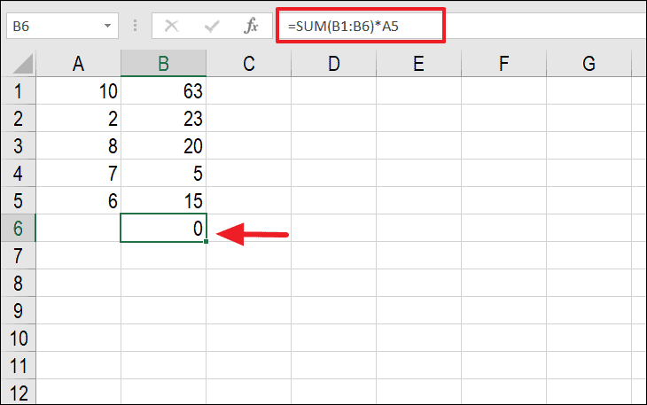
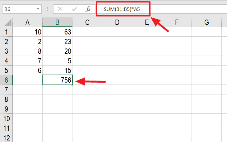
For example, if you have a formula in cell B6 as =SUM(B1:B6)*A5, and it’s causing a circular reference, you can fix it by changing the formula to exclude B6: =SUM(B1:B5)*A5.
This adjustment removes the circular reference, and cell B6 will display the correct result.
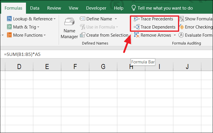
When dealing with complex formulas, you can use the ‘Trace Precedents’ and ‘Trace Dependents’ tools to visualize cell relationships and identify circular references.
These tools can be found under the ‘Formulas’ tab in the ‘Formula Auditing’ group.
Trace Precedents
This feature shows all the cells that a formula depends on. Select the cell with the formula causing the issue and click ‘Trace Precedents’. Blue arrows will point to the cells that are direct inputs to the formula.
In the example below, the blue arrows indicate that cell B6 depends on cells B1 through B6 and A5. Since B6 is included in its own calculation, it creates a circular reference.
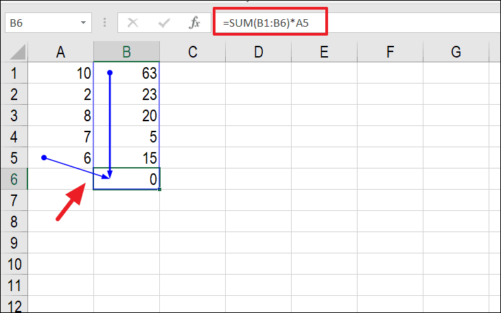
By adjusting the formula to exclude B6, you eliminate the circular reference.
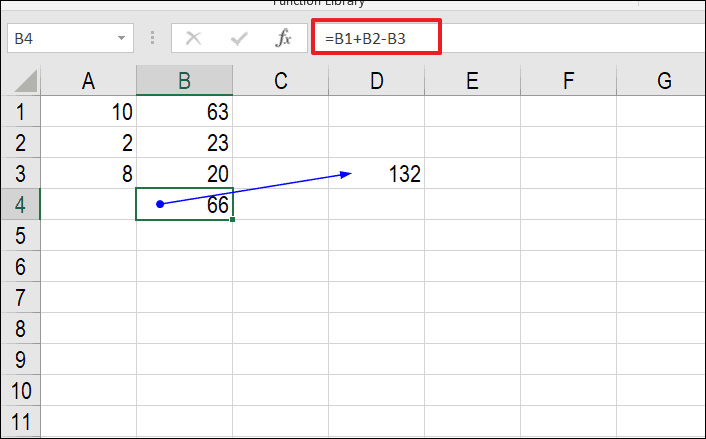
Trace Dependents
‘Trace Dependents’ shows all the cells that rely on the selected cell. Selecting a cell and clicking ‘Trace Dependents’ will display arrows pointing to all formulas that use that cell’s value.
In the example below, cell D3 depends on the value in B4. The arrow indicates that changes in B4 will affect D3.
Intentionally Using Circular References
While generally discouraged, there are scenarios where circular references are intentionally used for iterative calculations. In such cases, enabling iterative calculations allows Excel to compute results that rely on successive approximations.
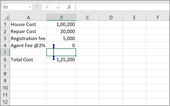
Example: Calculating a commission that is a percentage of the total price, where the total price includes the commission.
First, ensure that iterative calculations are enabled in Excel.
Suppose you’re calculating the total cost of a house purchase, including a 2% agent commission based on the total cost. This creates a circular reference because the total cost depends on the commission, which in turn depends on the total cost.
In cell B6, calculate the total cost:
=SUM(B1:B4)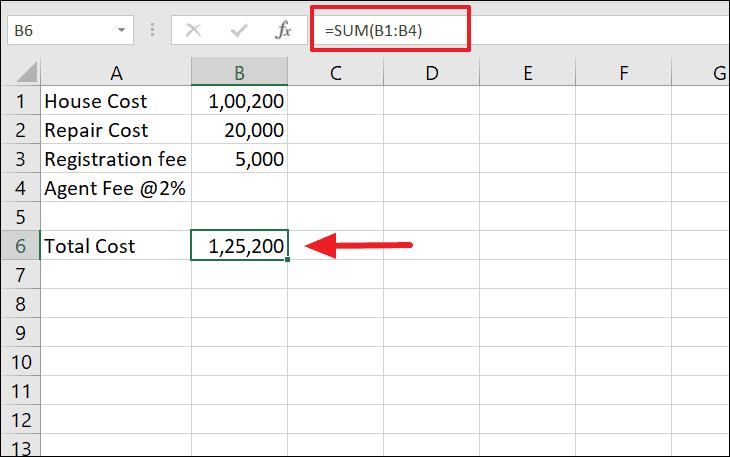
In cell B4, calculate the agent’s fee as 2% of the total cost:
=B6*2%This setup creates a circular reference between B4 and B6.
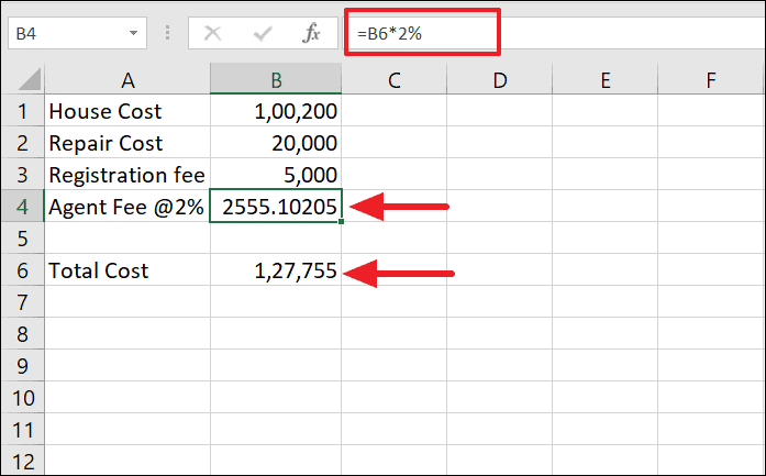
With iterative calculations enabled, Excel will compute the values through repeated approximations until the results converge, providing an accurate total cost including the commission.
If iterative calculations are not enabled, Excel will display a warning and may not compute the correct values.
Understanding and managing circular references in Excel is essential for ensuring accurate calculations. By learning how to identify and resolve these references, you can maintain the integrity of your data and utilize Excel’s capabilities effectively.


