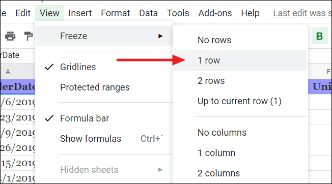
When handling large datasets in Google Sheets, important headers or labels can scroll out of view as you navigate through the sheet, making data tracking challenging. Freezing rows or columns keeps these key sections visible, enhancing data readability and navigation.
Freezing a column in Google Sheets
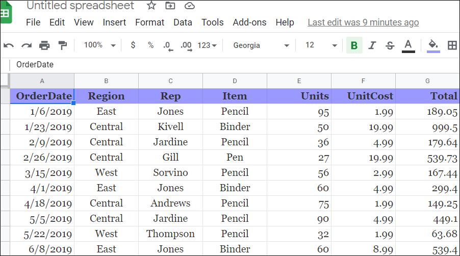
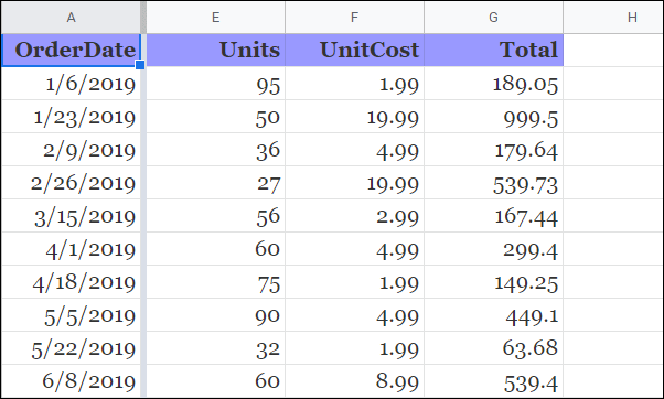
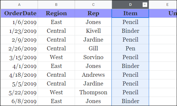
To illustrate how to freeze columns, we’ll use the following dataset in Google Sheets.
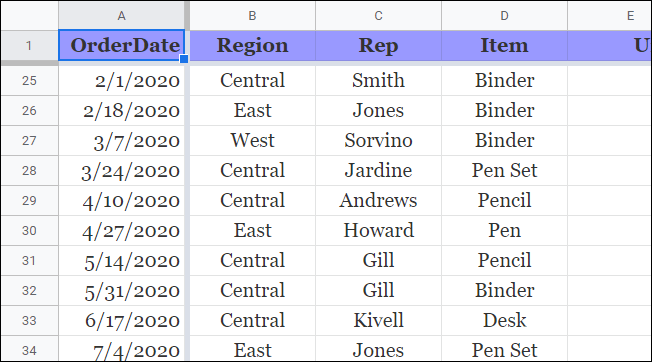
A gray divider will appear after the first column, indicating that it has been frozen.
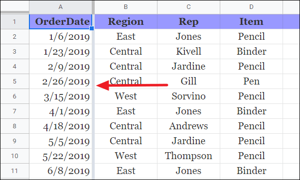
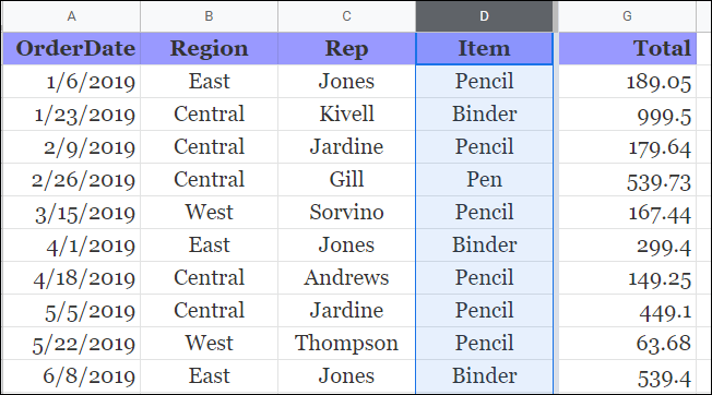
Now, when you scroll horizontally, the first column remains fixed. As shown below, after column ‘A’, the next visible column is ‘E’ because the columns between ‘B’ and ‘D’ have scrolled out of view, but the frozen column stays in place.
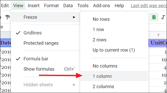
Freezing multiple columns in Google Sheets
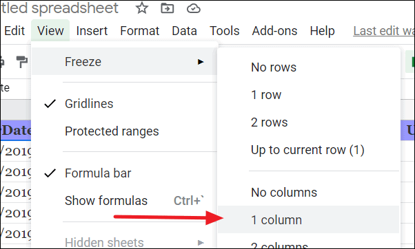
To freeze multiple columns, follow these steps:
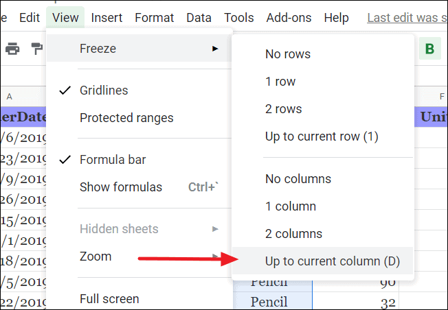
A gray divider will now appear after the selected column, showing that all columns up to that point are frozen.
Freezing a row and a column simultaneously
You can freeze both rows and columns at the same time using the Freeze options.
After these steps, two gray dividers will appear: one below the first row and one beside the first column, indicating both have been frozen. This setup keeps the first row and column visible as you scroll through your sheet.
Freezing rows and columns in Google Sheets ensures that important headers and labels remain visible, making it easier to navigate and analyze large datasets efficiently.