Transferring data between Google Sheets can significantly improve your workflow by automating data consolidation and ensuring consistency across multiple sheets. Rather than manually copying and pasting data, you can utilize the IMPORTRANGE() function to seamlessly import data from one sheet to another.
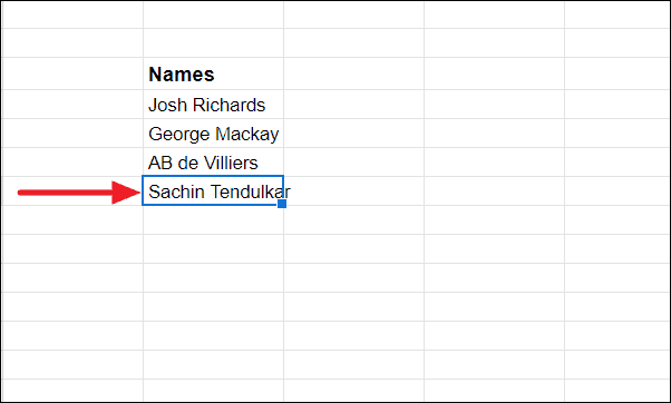
Import a cell from one Google Sheet to another
=IMPORTRANGE( to begin the function.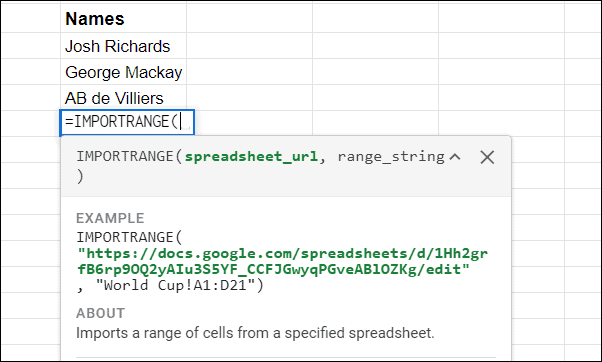
/d/ and /edit in the URL.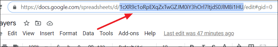
IMPORTRANGE() function, enclosed in double quotation marks. It should look like =IMPORTRANGE("spreadsheet_id".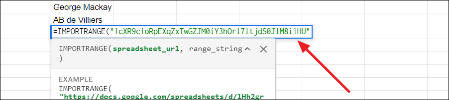
"Sheet1!B8". The full function should now look like =IMPORTRANGE("spreadsheet_id","Sheet1!B8").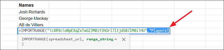
Tip: The sheet name (also called the sheet label) can be found at the bottom of the Google Sheets window. It is “Sheet1” by default, but you can rename it to something more descriptive by right-clicking the tab and selecting “Rename”. Renaming sheets helps prevent confusion when working with multiple sheets.

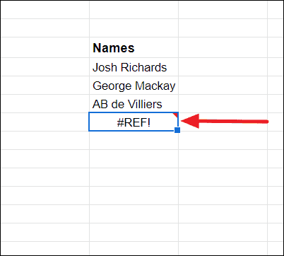
Enter. The cell should now display the imported data. If you see an error message, don’t worry; this is normal when connecting sheets for the first time.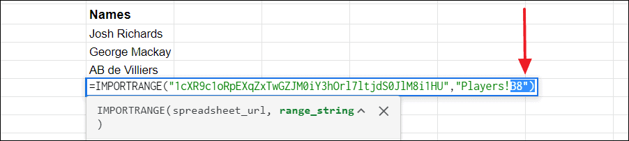
If an error occurs, it may look like this:
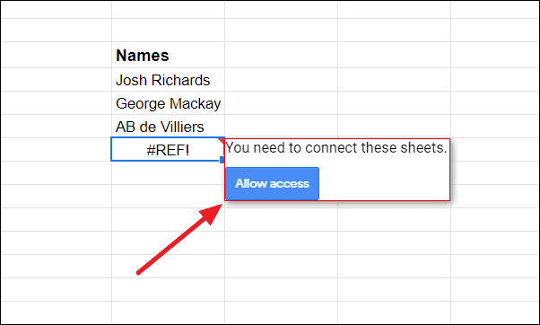
Once access is granted, the data from the specified cell in the source sheet will appear in your destination sheet.
Import a column from one Google Sheet to another
=IMPORTRANGE(. Include the spreadsheet ID as before."Sheet1!B1:B100", where B1 is the first cell and B100 is the last cell in the column range you wish to import. Adjust the ending cell according to your data.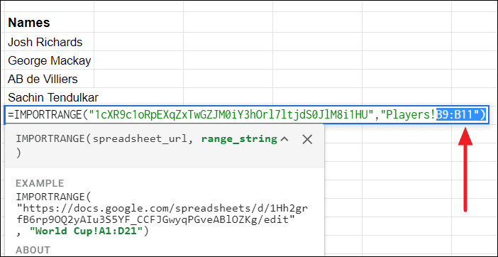
Enter. If prompted, allow access to the source sheet. The specified column data will now populate in your destination sheet, starting from the selected cell.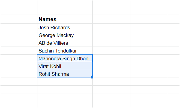
Import an entire table from one Google Sheet to another
IMPORTRANGE() function with the spreadsheet ID."Sheet1!A1:D10" will import all data in the rectangle from cell A1 to D10.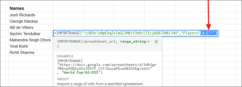
Enter. After granting access if prompted, the entire table will be imported into your destination sheet, maintaining the original formatting and structure.
By using the IMPORTRANGE() function, you can efficiently manage and synchronize data across multiple Google Sheets, ensuring that any updates made in the source sheet are automatically reflected in the destination sheet without manual intervention.