
When managing an accounting ledger or a large product list, you may need to highlight or shade alternate rows in your worksheet to make it easier to read and sort data. Highlighting alternate rows help distinguish the different rows from monotonous data and makes it user-friendly.
If you were to manually select every other row one by one and add colors to them, it would be time-consuming and tiresome. Instead, you can have Excel color alternate rows automatically.
Shading a different color for every other row or highlighting alternate rows can be done using several different automatic methods, including Conditional formatting, built-in table styles, formulas, and VBA macro. In this tutorial, we will cover all four methods and more.
Manually Highlight Every Other Row in Excel
The simplest way to highlight or shade color every other row in an Excel table is to manually select rows and fill in them with the color of your choice.
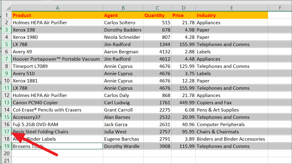
Hold down the Ctrl key and click on the row numbers on the left-hand side of every other row.
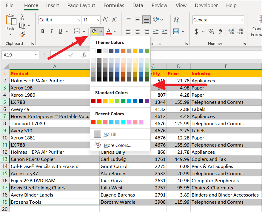
After selecting all the rows, go to the ‘Home’ tab and click the arrow next to the ‘Fill Color’ button (paint bucket icon) in the Font Group. From the drop-down menu, choose the color of your choice.
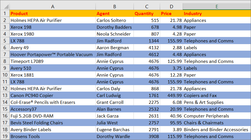
You got your alternate rows highlighted:
This is a time-consuming process. If you prefer a more automatic method, try one of the following ways.
Highlight or Shade Alternate Rows using Table Styles
The easiest and quickest way to highlight every other row in Excel is by applying predefined Excel table styles. Excel has a large number of built-in table styles or table templates that you can use to achieve this. Let us show you how to do that:
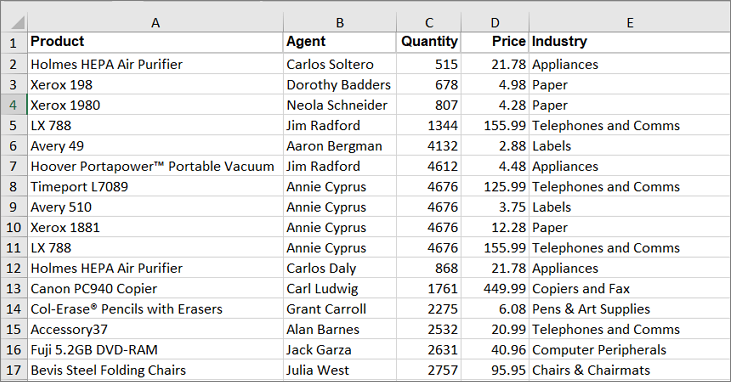
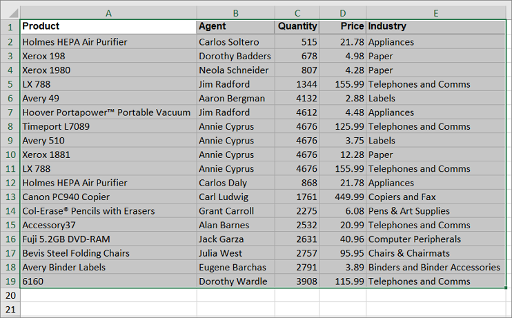
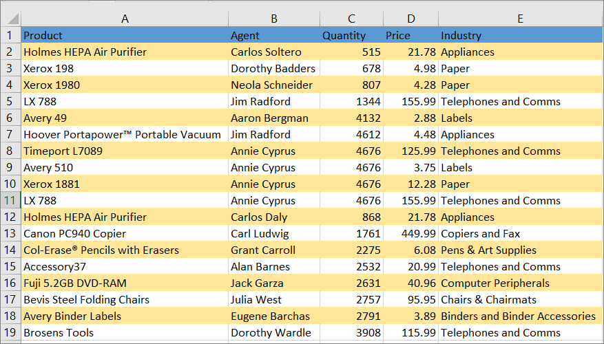
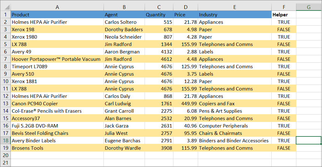
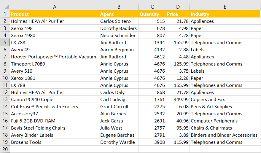
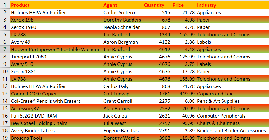
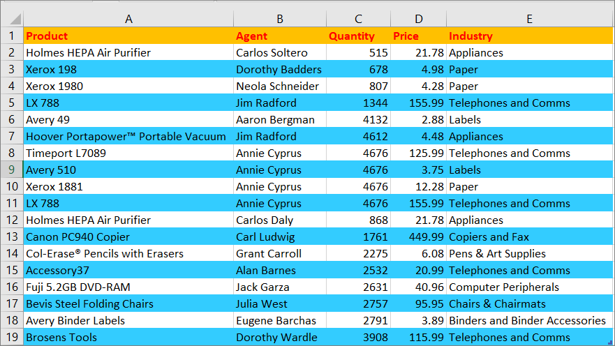
Suppose, you have the below dataset where you want to highlight the alternate rows.
First, select the range of cells where you want to alternate color rows or any cell in the dataset.
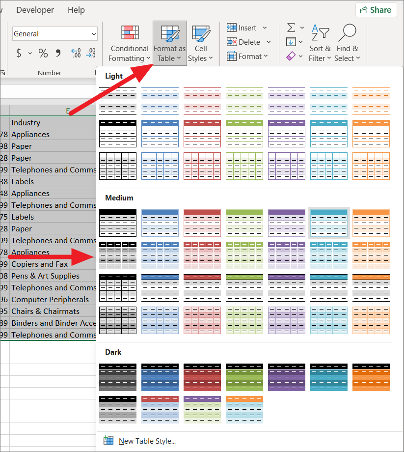
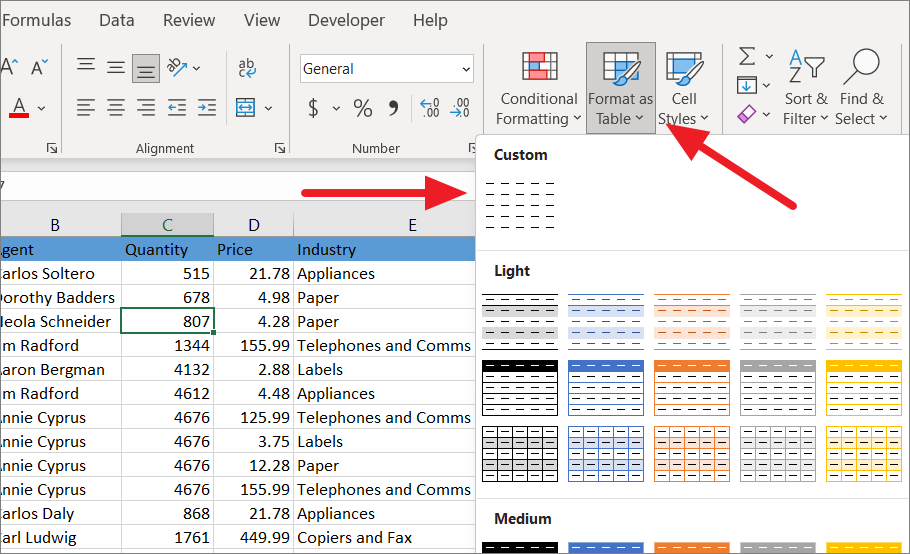
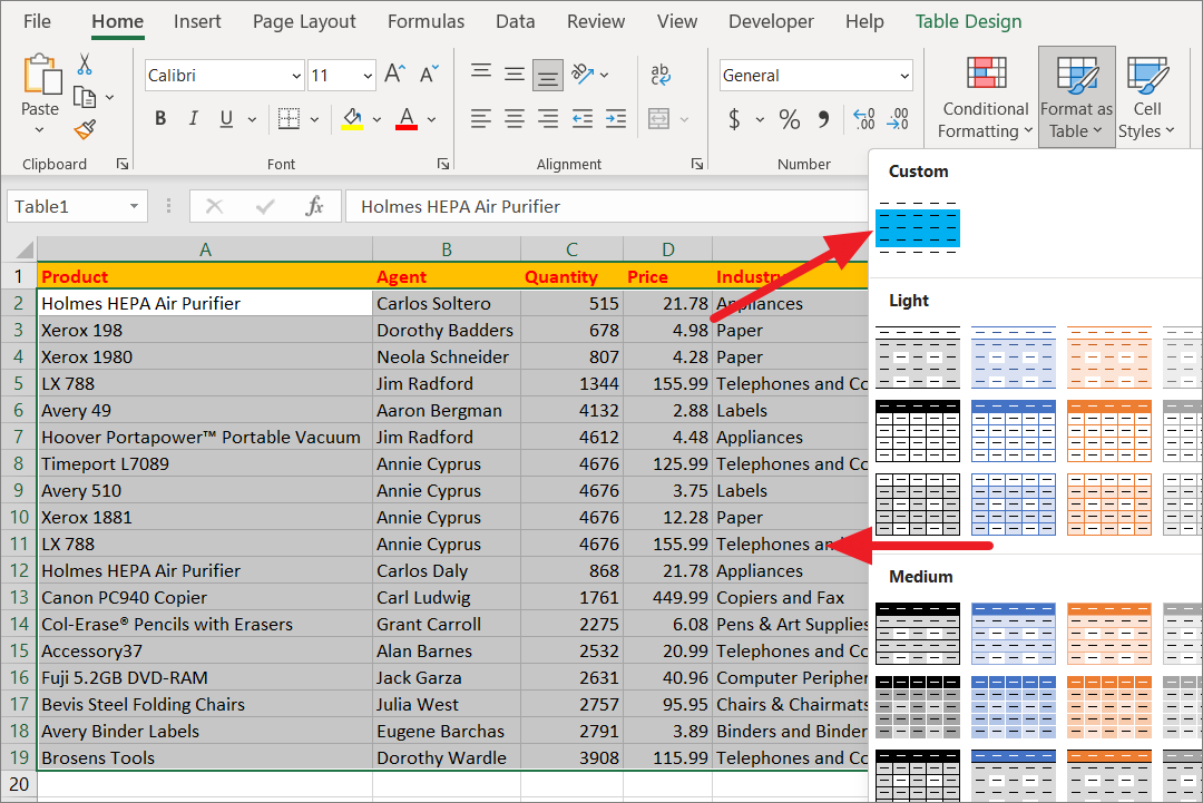
From the ‘Home’ tab, click the ‘Format as Table’ button in the Styles section. In the drop-down menu, select any of the formatting styles with banded rows (style with alternate row shading) from Light, Medium, and Dark sections.
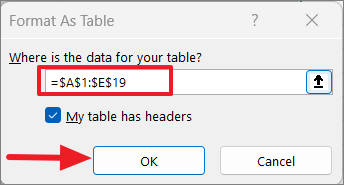
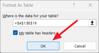
After selecting the style, a Format As Table dialog will pop up to confirm the range where you want to apply this table formatting. If the range is correct, click ‘OK’, if not change the range in the field and click ‘OK’. Before you click ‘OK’, tick the ‘My table has headers’ option if your data contains headers.
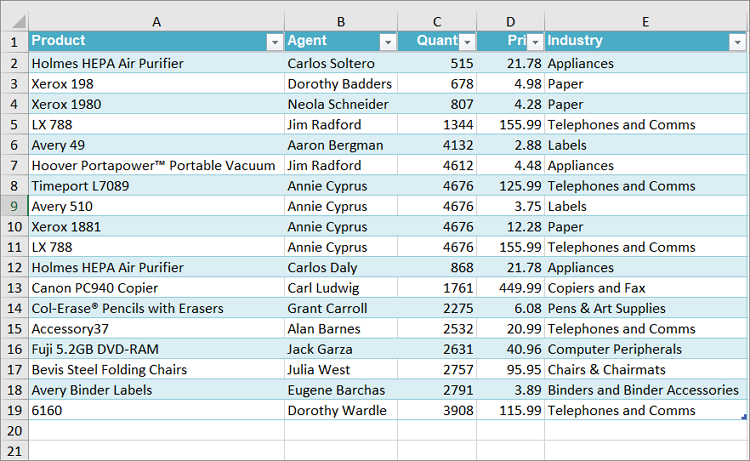
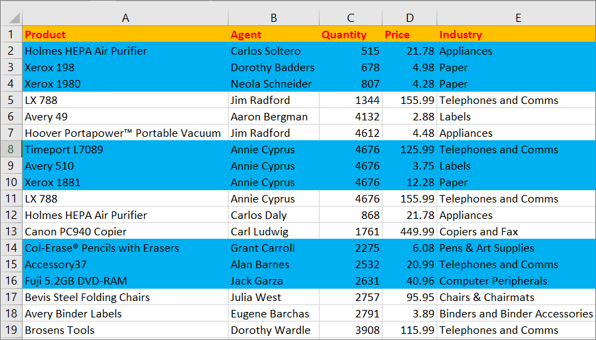
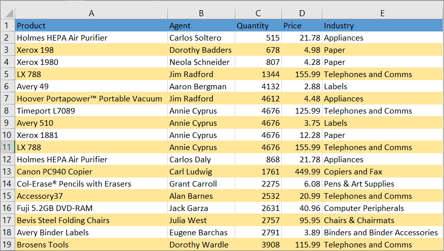
This will convert the range into a table, apply the selected table format, and color your alternate rows as shown below. In addition to this, it will also make your table dynamic with table functionalities, like sorting, filtering, etc.
If you don’t like the current color shading, click the ‘Format as Table’ drop-down again and choose a different table style.
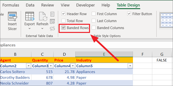
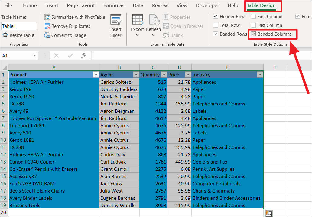
If the alternate rows are not highlighted even after formatting the table with table style, go to the ‘Table Design’ or ‘Design tab’ (which will only appear if the table is selected) and make sure that the ‘Banded Rows’ checkbox is checked in the Table Style Options group.
Create Custom Table Formatting for Shading Alternate Rows
Although there are several pre-built table styles in Excel to choose from, if you don’t like any of them, you can still create your own table style and use it to color alternate rows. Also, Excel only has built-in formatting styles to shade alternate rows but not columns. But with custom formatting, you can also highlight alternate columns. Let us see how.
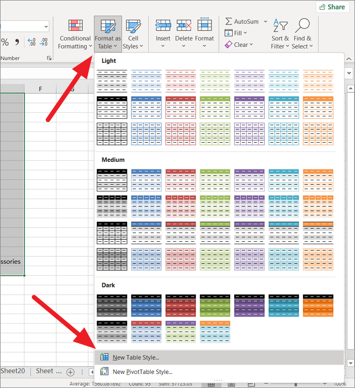
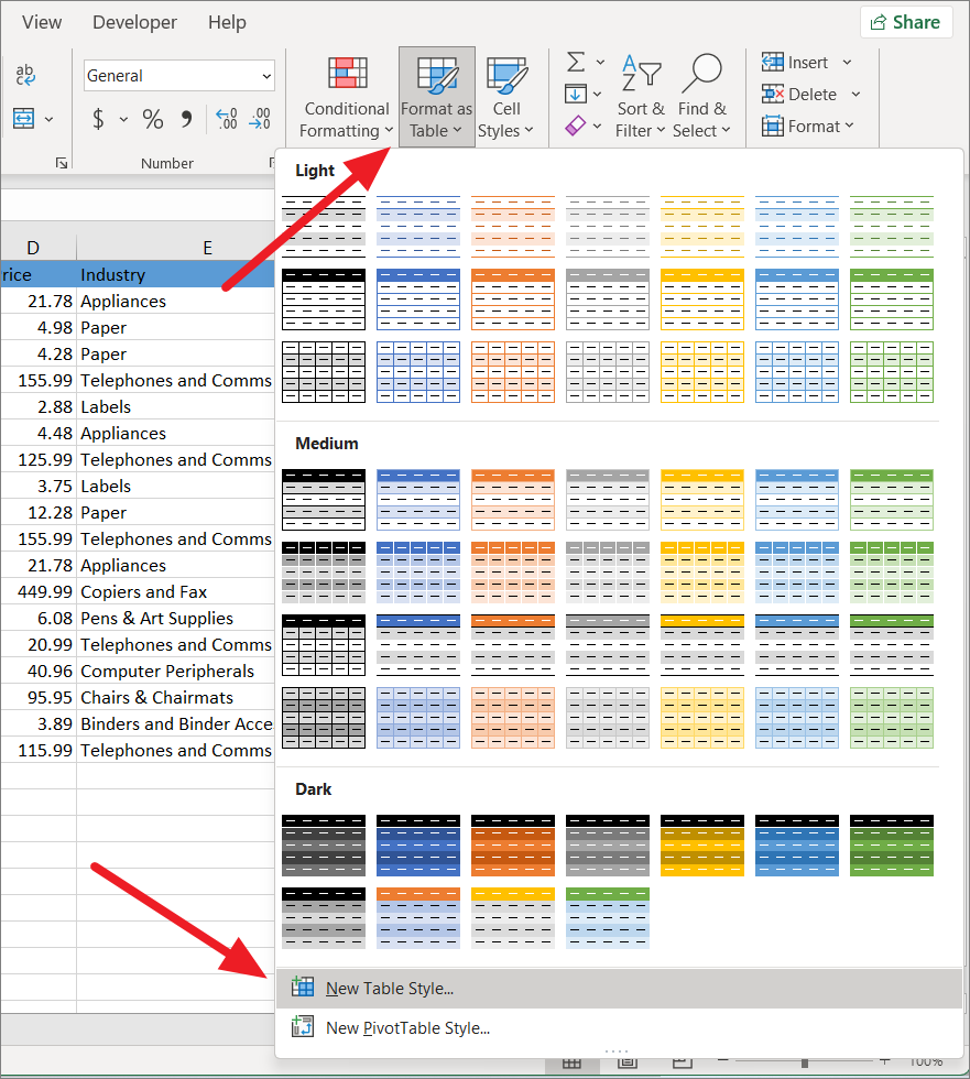
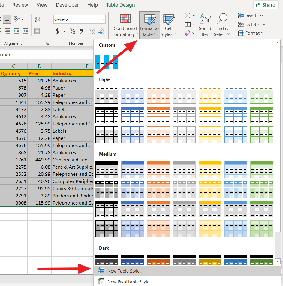
To create a custom table style, go to the ‘Home’ tab and select the ‘New Table Style…’ option from the bottom of the ‘Format as Table’ dropdown menu.
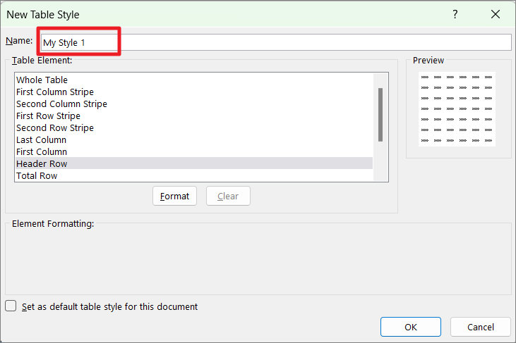
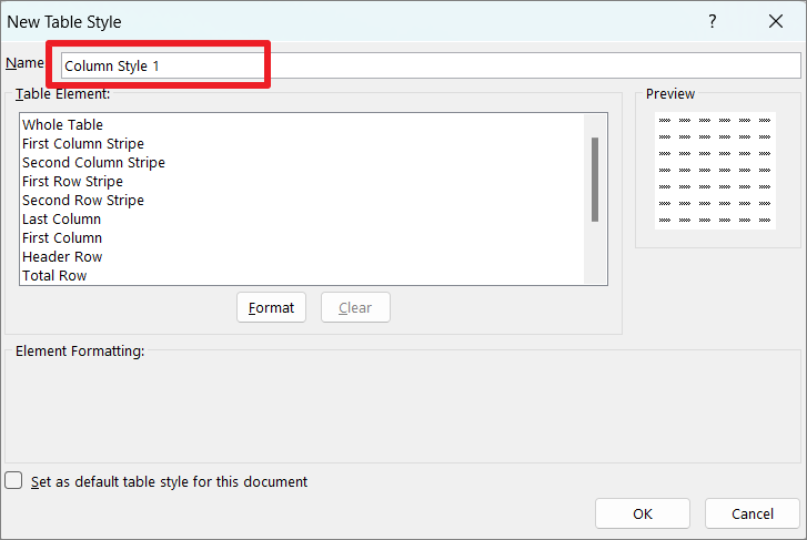
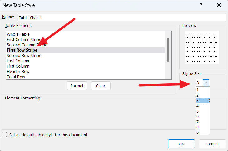
In the New Table Style dialog, give a name to the custom table style or continue with the default name. Under the Table Element, you can choose various table elements of the table and format them however you want.
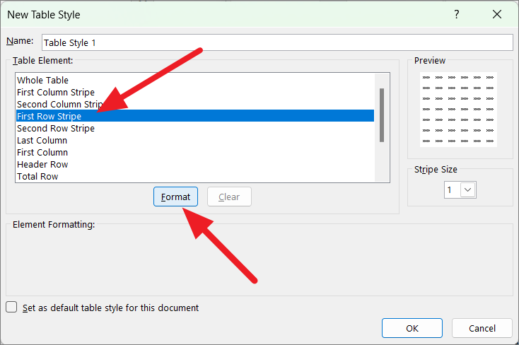
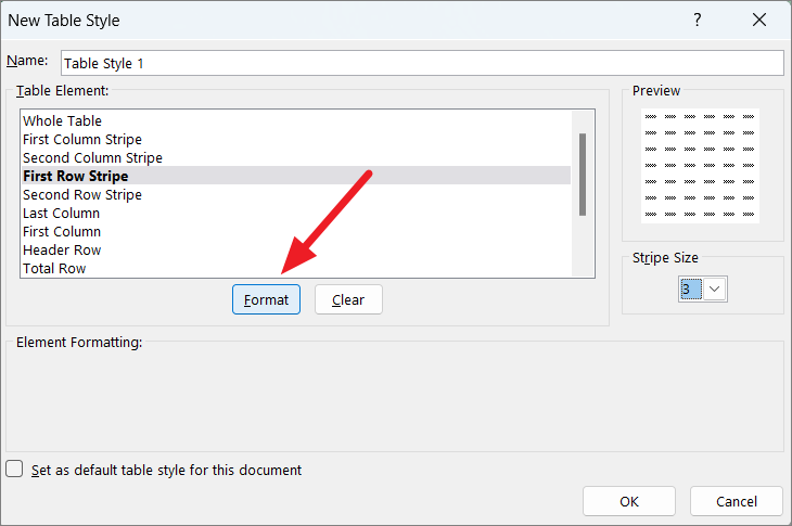
To highlight every other even-numbered row starting from the first row of the table under the header (2, 4, 6, etc.), select the ‘First Row Stripe’ element and click ‘Format’.
To highlight every other odd-numbered row starting from the second row of the table under the header (3, 5, 7, etc.), select the ‘Second Row Stripe’ element and click ‘Format’.
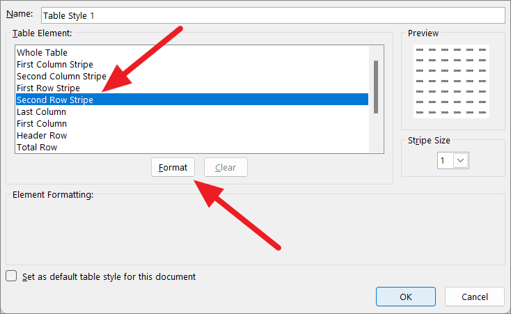
Either way, this will open the Format cells window where you can fine-tune your table’s style however you like with the formatting options.
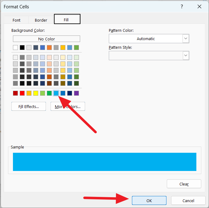
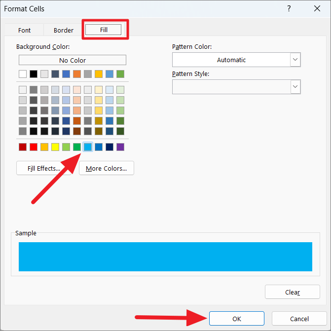
To highlight the alternate rows with colors, go to the ‘Fill’ tab and choose whatever color you want your alternate rows to have, and click ‘OK’. To get more colors, click the ‘More Colors’ button. You can also add gradient effects by clicking the ‘Fill Effects…’ button.
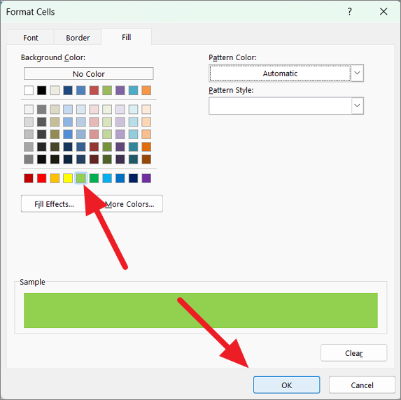
If you want, you can also customize pattern color and style using the two drop-down menus.
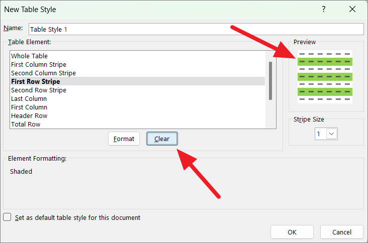
After selecting formatting, you can see the preview of the formatting in the Preview box and if you don’t like it, click the ‘Clear’ button to remove the formatting.
Now, add a different color scheme to the header row to make it distinct. To do that, select the ‘Header Row’ option, and click on ‘Format’.

Then, select a different color scheme for the header row and click ‘OK’.
If you want to use this table formatting frequently, check the ‘Set as default table style for this document’ to make this the default style. After finalizing the color scheme, click ‘OK’ to save this table style.
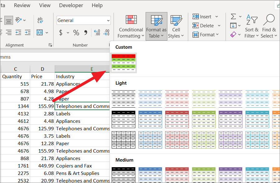
Once you created a custom table style, it will be added to the Custom section of the ‘Format as Table’ menu. Now select any cell in the range or the entire table range and choose your custom table formatting from the ‘Format as Table’ menu.
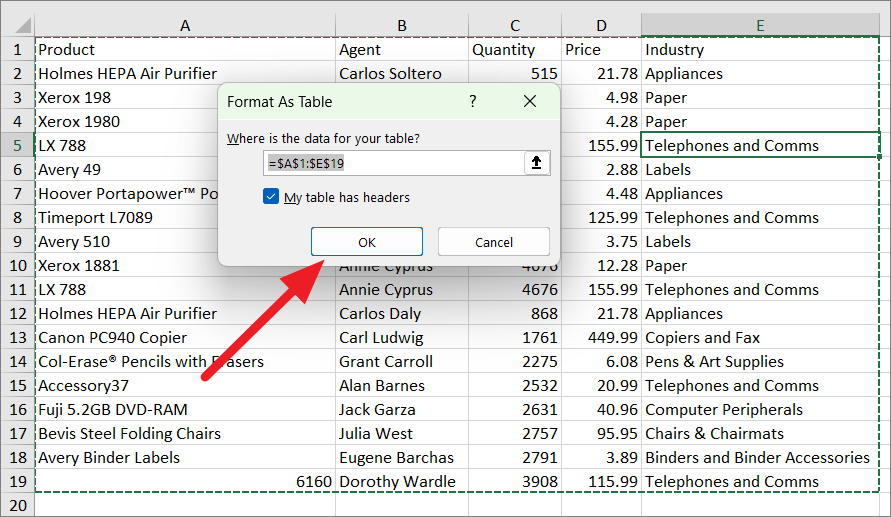
Then, confirm the range in the Format As Table box and click ‘OK’.
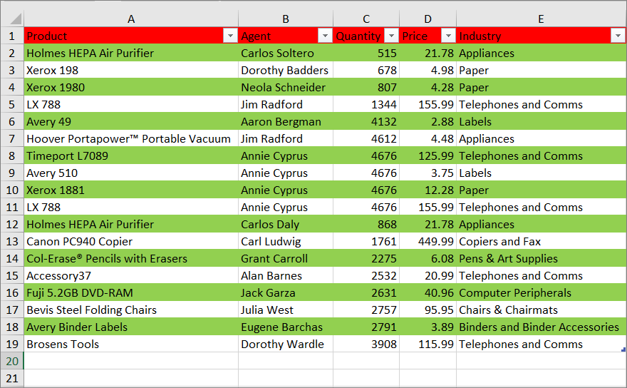
Now, every other row will be highlighted with your customized table style.
The advantage of using the table style method to highlight alternate rows is that whenever you add rows to the range or remove rows from the range, Excel will automatically shade those alternate rows with the color banding (as shown below). Now, even if you sort, filter or move the data within the table, color banding will remain unchanged.
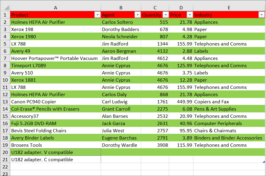
If you only want the alternate row color banding without the table functionality, you can convert the table back to a range. Here’s how:
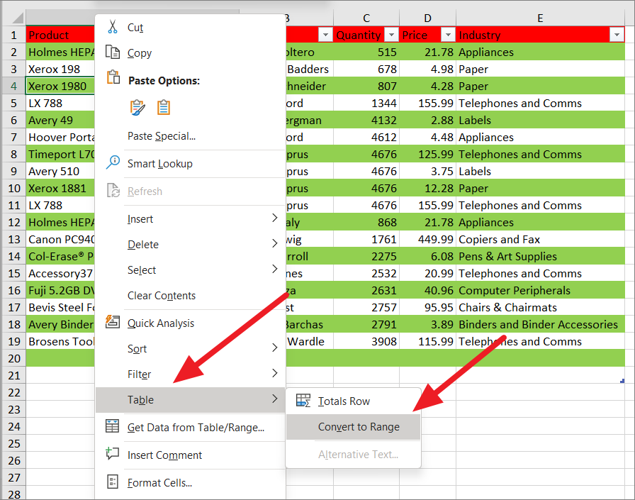
Select any cell in the table, right-click on it, hover over ‘Table’ from the context menu, and then select the ‘Convert to Range’ option.
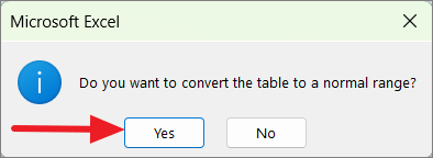
In the confirmation box, click ‘OK’,
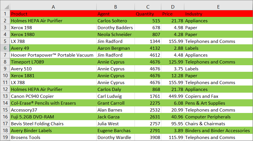
Now, the table will be converted to a range but the color shading or stripes will remain in the range.
However, if you move, sort, or filter specific cells or entire rows within the range, the color shading will go along with the row, disrupting the alternate highlight.
Highlight Every Other Column in Excel
Excel’s pre-built table styles (also called zebra striping) can only be used to highlight every other row but there are no preset table styles to highlight alternate columns. So if you need to highlight alternate columns, you can only do it with your custom table style. To do this, follow these instructions:
From the ‘Home’ tab, click the ‘Format as Table’ button in the Styles group and select the ‘New Table Style…’ option.
In the New Table Style dialog box, enter a name for your new custom style.
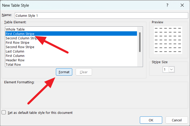
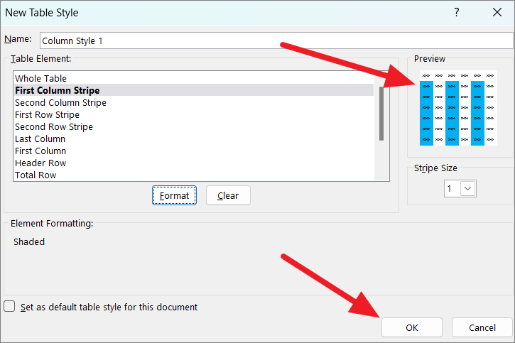
To highlight every other column starting from the first column (column A) of the table (A, C, E, etc.), select the ‘First column Stripe’ element and click ‘Format’.
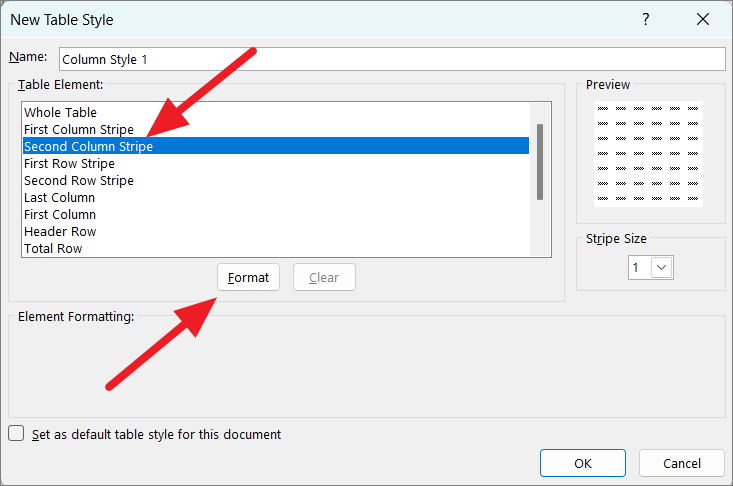
To highlight every other column starting from the second column (column B) of the table (B, D, F, etc.), select the ‘Second column Stripe’ element and click ‘Format’.
In the Format cells dialog, you can customize the table style with various formatting options however applying fill color is enough to highlight rows in the table. To do this, go to the ‘Fill’ tab and choose a fill color. Then, you can also set fill effects and pattern style if you want. After that, click on ‘OK’.
Then, confirm the formatting in the Preview box and click ‘OK’ to save the custom table style.
After saving the custom table style, select the range or any cell in the table, and choose your new custom table style from the ‘Format as Table’ menu.
Then, confirm the range in the ‘Format As Table’ box and click ‘OK’.
If you still don’t see your alternate columns highlighted, select any cell in the table, and go to the ‘Table Design’ or ‘Design’ tab. And make sure that the ‘Banded Columns’ checkbox in the Table Style Options is checked.
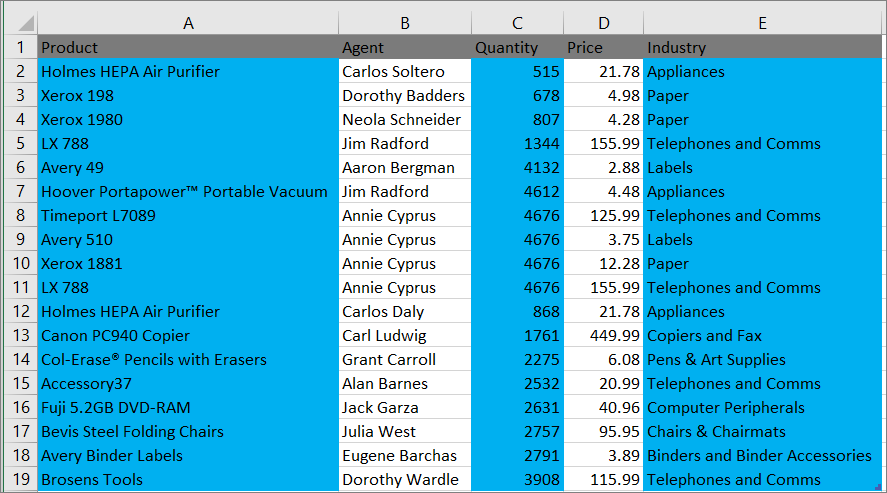
Now you got your alternate columns highlighted as shown below.
Highlight Every Other nth Row
In case you want to highlight every 3rd, 4th, or any other number of rows, you can change the stripe size in the table formatting.
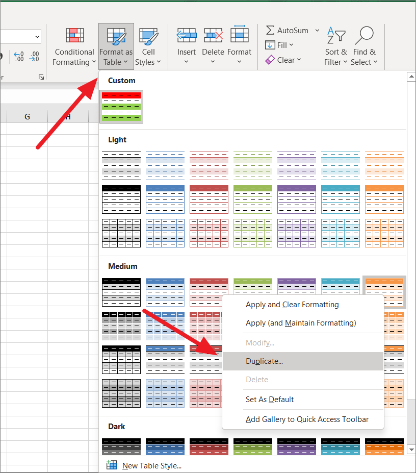
To do this, open the ‘Format as Table’ menu and right-click any table style option (Custom or built-in) that you want to apply, and select ‘Duplicate’ to edit it.
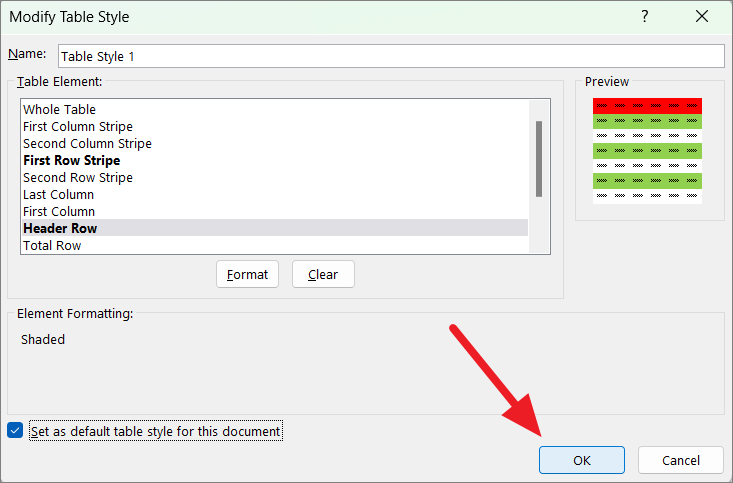
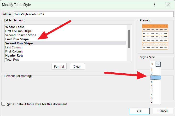
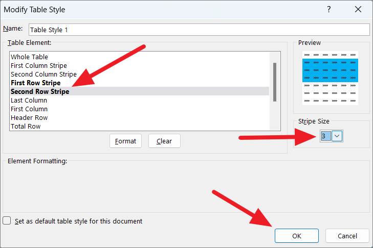
This will open the ‘Modify Table Style’ dialog box. Here you can change the stripe size to customize the shading area.
Now, select the ‘First Row Stripe’ option from the list and ensure the Stripe Size is ‘1’.
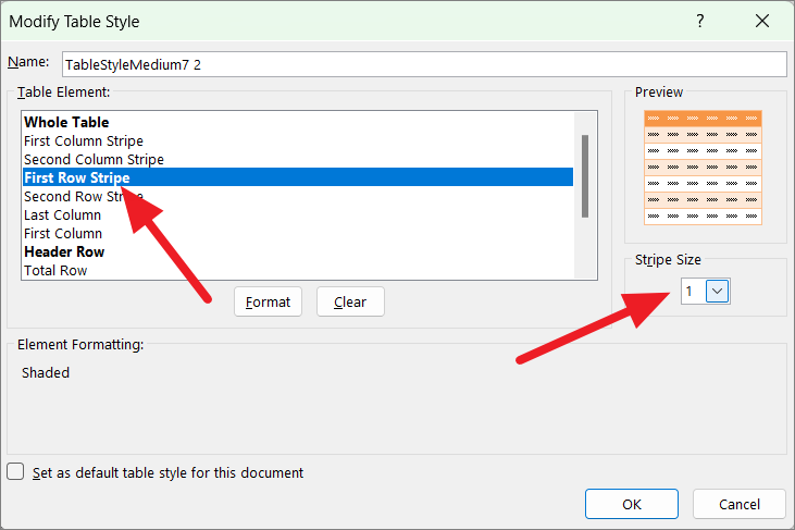
After that, select the ‘Second Row Stripe’ option and select the number of rows you want to skip from the ‘Stripe Size’ drop-down. For example, if you want to highlight every 4th row, you have to skip 3 rows in between, so, we selected ‘3’. And make sure not to add any formatting to the ‘Second Row Stripe’ element.
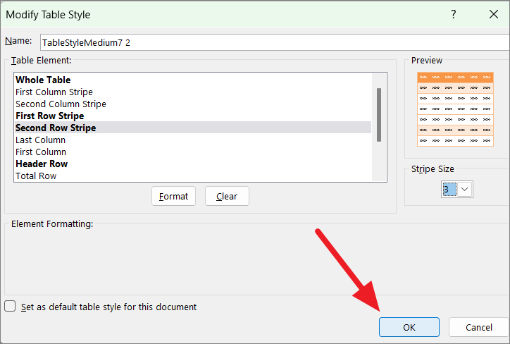
Then, give a name to the style and click ‘OK’. to save this formatting as a new custom table style.
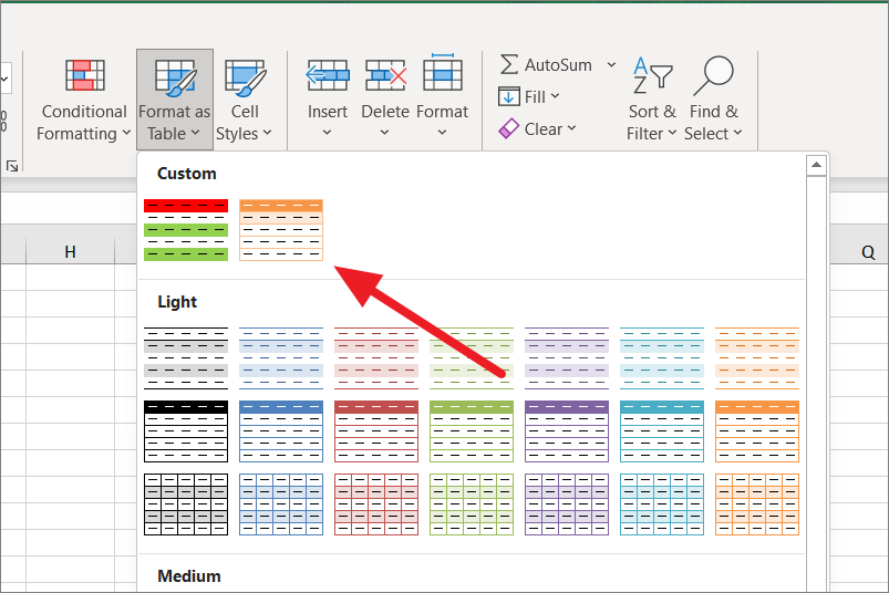
The newly customized table style will be added to the list of table styles. Now, select any cell within the table and select the newly modified table style under the ‘Format as Table’ menu.
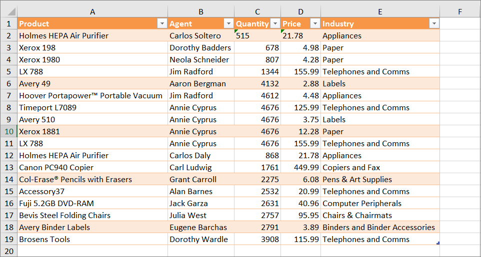
As you can see only every 4th row is highlighted with the color scheme.
Highlight Alternate Groups of Rows
You can also create custom table styles to highlight alternate groups of rows instead of just single alternate rows in an Excel table. For example, to highlight every other group of three rows, follow these steps below:
From the ‘Home’ tab, click the ‘Format as Table’ drop-down menu in the Styles section and select the ‘New Table Style’ option.
In the New Table Style dialog, name the table style and select the ‘First Row Stripe’ element, and set the ‘Stripe size’ to the number of rows you have in each banded group. Here, we are selecting ‘3’.
Next, click the ‘Format’ button to select the format you want to apply.
In the ‘Fill’ tab, choose the color you want to apply to the banded group of rows, and click ‘OK’.
Then, select the ‘Second Row Stripe’ and set the ‘Stripe Size’ to ‘3’. Then, click ‘OK’ to save the table style.
After that, select the range to apply the formatting and choose your custom table style from the ‘Format as Table’ menu.
This will color every other 3 rows in the table as shown below.
How to Highlight Every Other Row using VBA Script
Although it is not as simple as the above methods, if you prefer coding, you would probably want to use VBScript to shade or highlight every other row in Excel. Here’s how you can do that:
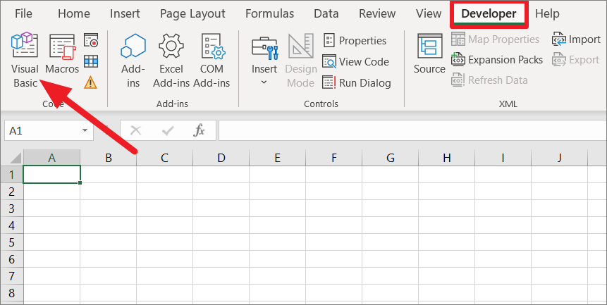
To open the Visual Basic for Applications window, go to the ‘Developer’ tab and click the ‘Visual Basic’ option from the ribbon or press Alt+F11.
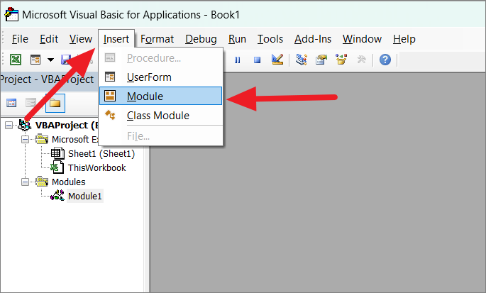
In the VBA window, click the ‘Insert’ tab, then select the ‘Module’.
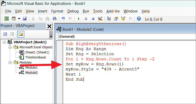
Now, type or copy-paste the below code into the new module window:
Sub highlight_everyother_rows()
Dim Rng As Range
Set Rng = Selection
For i = Rng.Rows.Count To 1 Step -2
Set myRow = Rng.Rows(i)
myRow.Style = "40% - Accent5"
Next i
End Sub
In the code, you can use any style (like “Accent1”, “Accent2”, “Accent3” etc.) from the Styles section of the ‘Home’ tab to highlight the rows.
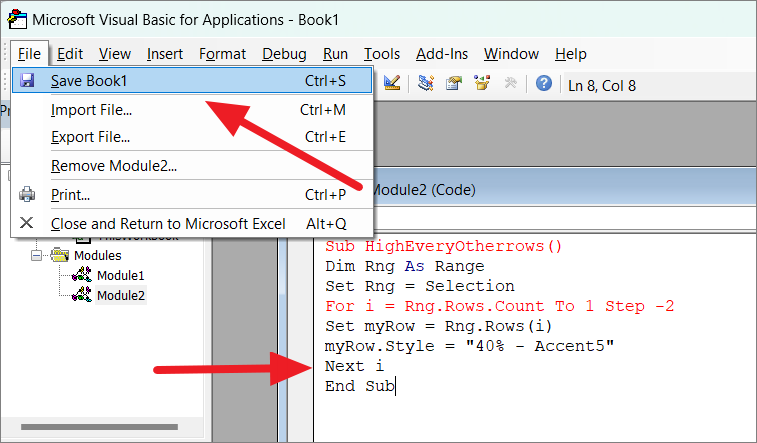
After entering the code, click ‘File’ and select ‘Save’ to save this module as a macro which can be run any time you want.
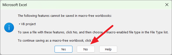
However, you can save macros in a normal excel file, you have to save the module in a macro-enabled Excel file. When you try to save the macro in a macro-free file, you will see the following warning box. Here make sure to select ‘No’.
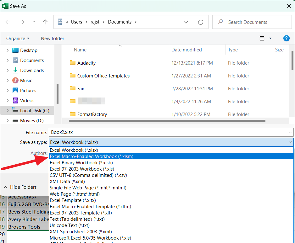
In the Save As window, choose ‘Excel Macro-Enabled Workbook (*.xlsm)’ format from the ‘Save As type’ drop-down and click ‘Save’.
To run the macro, follow these steps:
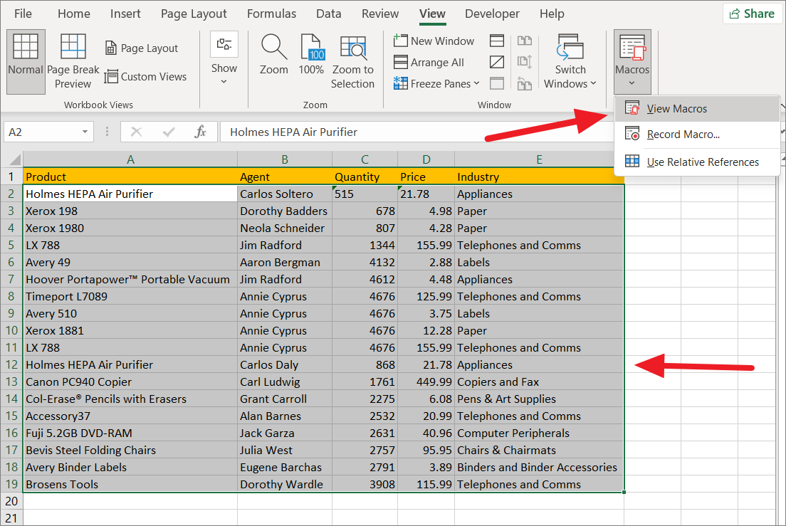
First, select the range where you want to highlight the alternate rows. If your table has a header, don’t include the header in the selection. Then, switch to the ‘View’ tab, click ‘Macros’ from the ribbon, and select the ‘View Macros’ option from the menu.
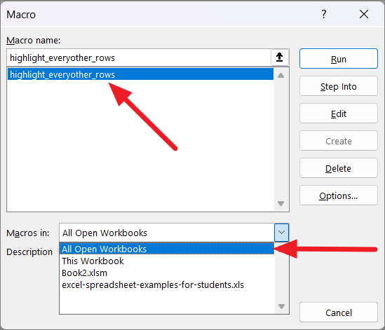
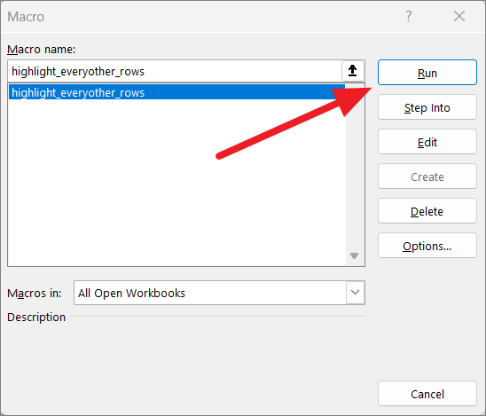
This will open the Macro dialog box. Select the macro for highlighting alternate rows from the box. Then, from the ‘Macros in:’ drop-down, choose whether you want to run this macro in ‘All Open Workbooks’, only ‘This Workbook’, or a specific workbook. Here, we are selecting ‘All Open Workbooks’.
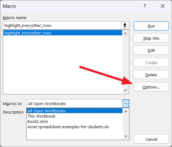
The advantage of using this method is that you can set shortcuts for the macro and then you can use that shortcut to run macro and highlight alternate rows whenever you want.
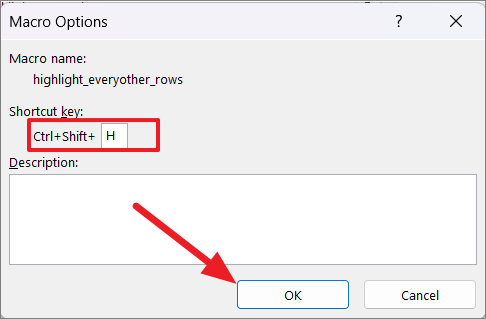
To do this, click the ‘Options…’ button in the Macro dialog box.
In the Macro Option, set your desired shortcut key under the ‘Shortcut Key:’ section for this macro. Then, click ‘OK’.
Then, click the ‘Run’ button in the Macro dialog window or close this dialog window and simply press the shortcut key you set.
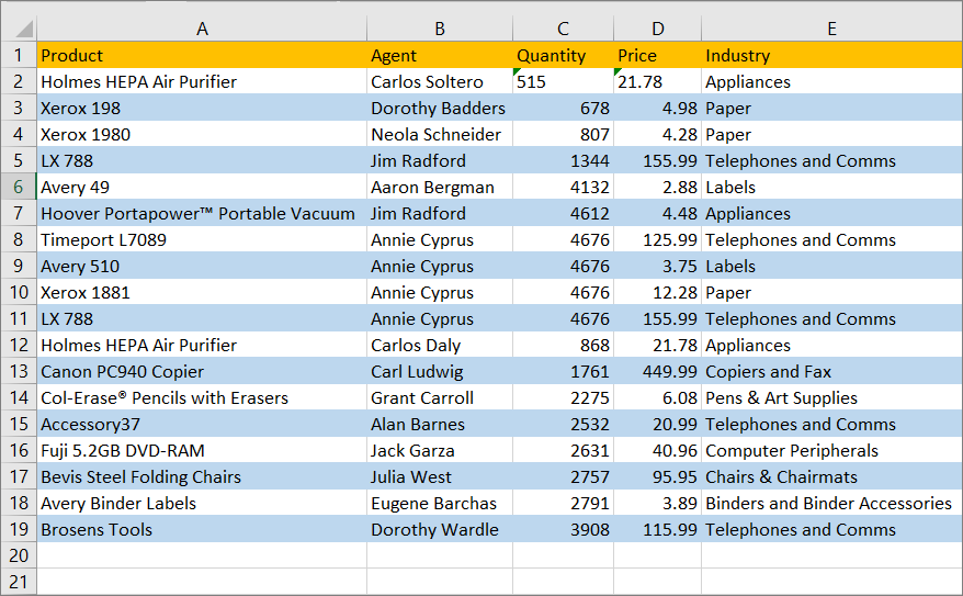
Now, every alternate row in your selected range will get highlighted as shown below.
Highlight Alternate Rows Using Filter with ISEVEN/ISODD and ROW Function in Excel
Another way you can highlight every other row in a table involves filtering, ISEVEN/ ISODD, and ROW functions. We need to create a helper column next to the data set. Then, you can use the combination of ISEVEN/ISODD and ROW function to return TRUE for alternate rows. After that, we need to filter those TRUE values and highlight the corresponding rows.
Highlight Alternate Rows using ISEVEN and ROW functions
If you want to highlight only alternate even rows in a table, follow these instructions:
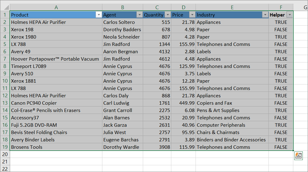
First, create a helper column right next to the data set (either to the left or right side of the table).
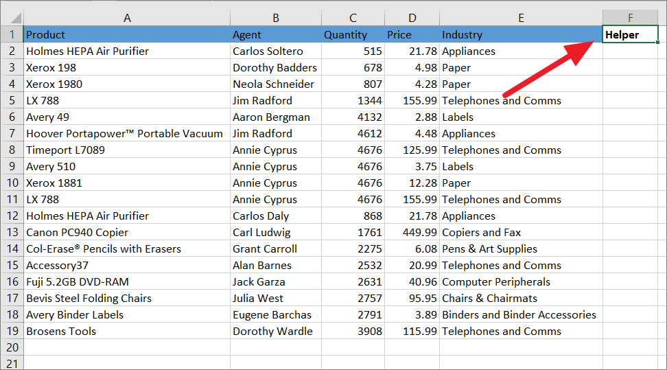
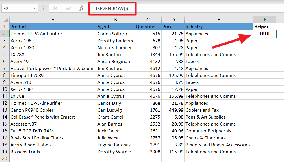
Now, enter the below formula in the first cell of the column:
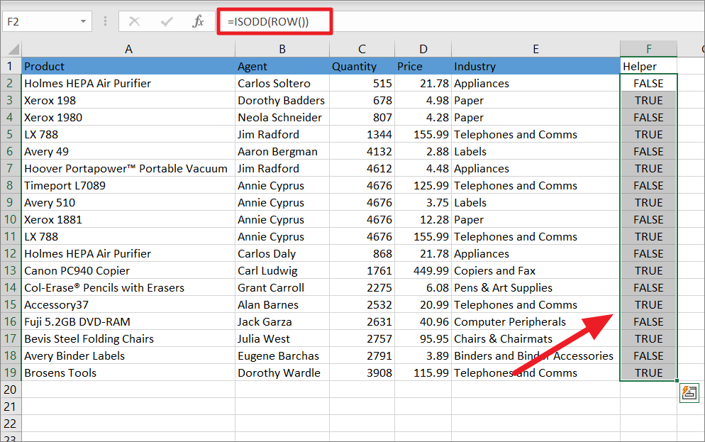
=ISEVEN(ROW())In the above formula, the nested ROW function returns the row number of the cell. Then, the ISEVEN function will produce TRUE if the returned row number is even or else FALSE if the number is odd. As you can see, it will return TRUE for row number 2 as it is an even number.
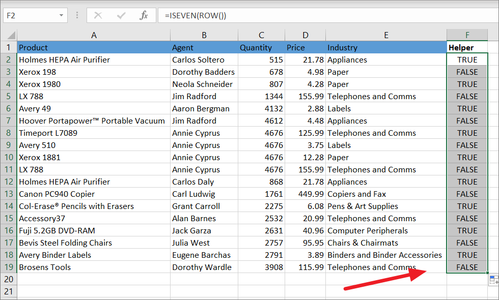
Then, click the fill handle and drag your mouse down to autofill the formula for the rest of the cells. Now, we got TRUE for each even row and FALSE for each odd row.
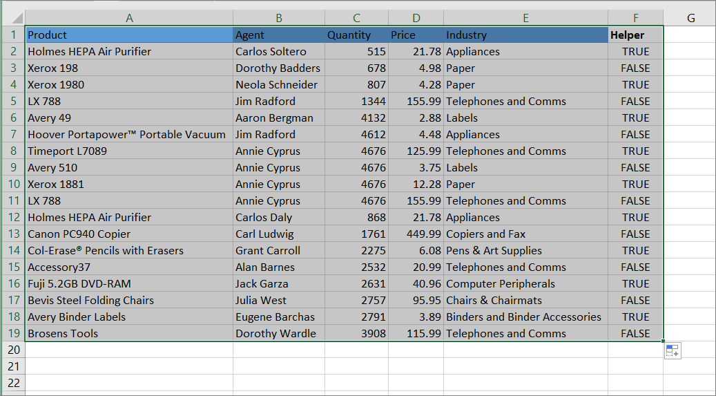
Next, select the range where you want to apply the filter including the helper column.
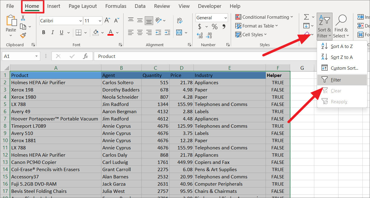
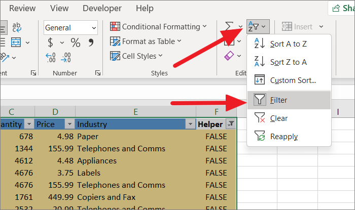
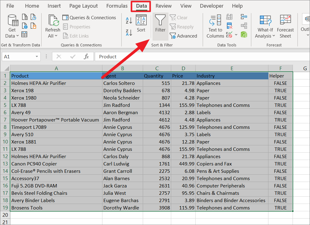
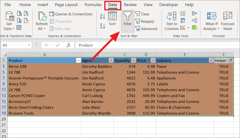
From the ‘Home’ tab, click the ‘Sort & Filter’ button in the Editing group, and select the ‘Filter’ option or press Ctrl+Shift+L. Alternatively, you can go to the ‘Data’ tab and select the ‘Filter’ from the Sort & Filter group.
Now, the Filter functionality will be applied to all the columns. You can see a little downward-facing arrow button next to each column header.
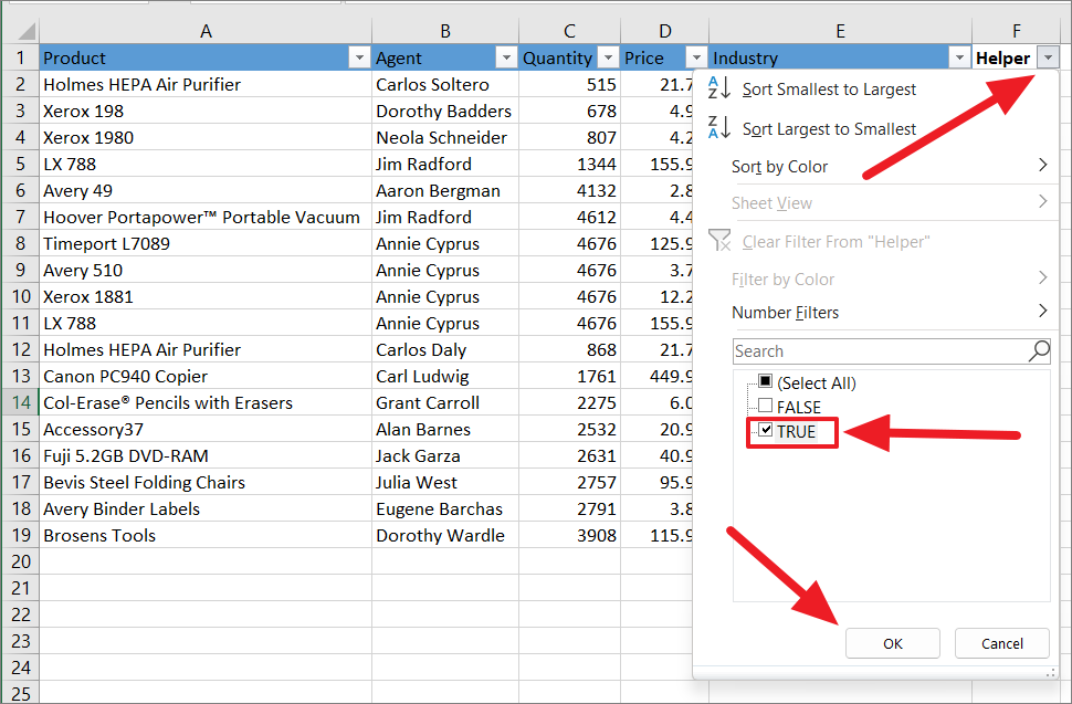
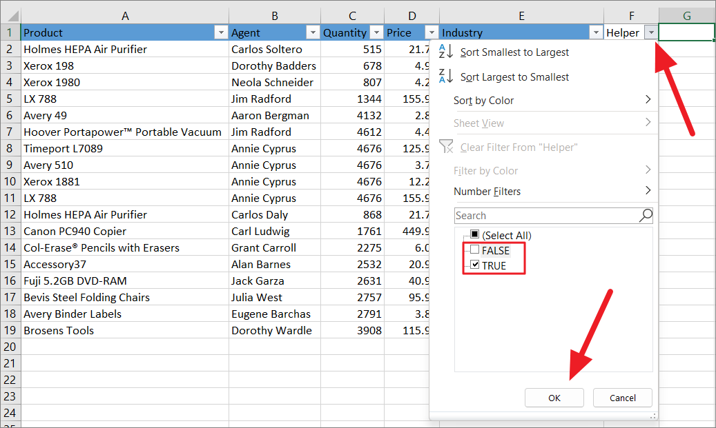
To highlight even-numbered alternate rows, click the little arrow on the Helper column, uncheck the ‘Select All’ checkbox, and check the ‘TRUE’ value. Then, click ‘OK’ to filter the TRUE values.
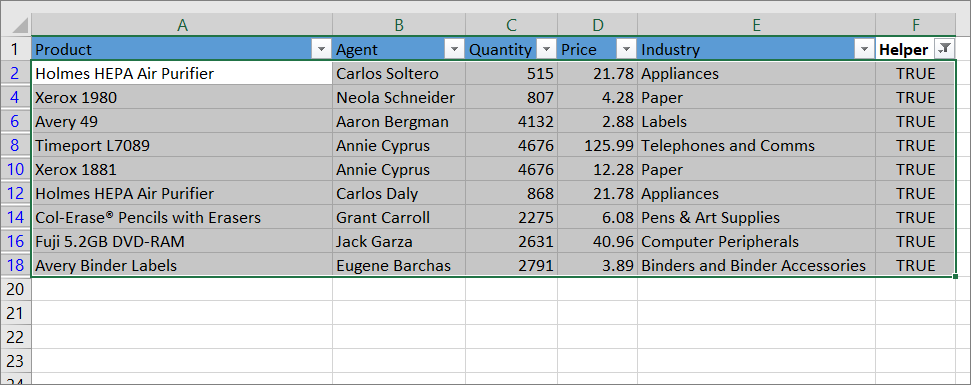
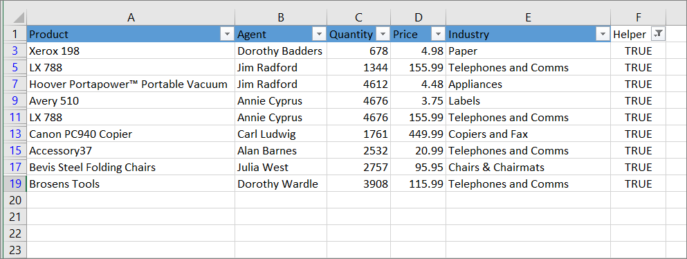
Now, all the column values will be filtered by the TRUE value where only the rows with TRUE (alternate even rows) will remain visible while others will be hidden.
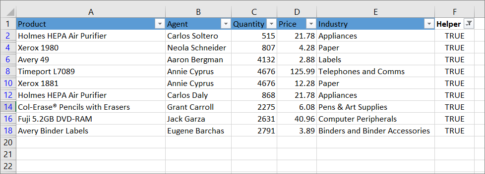
Now, select the filtered data except the header row.
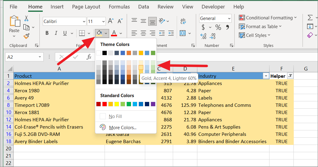
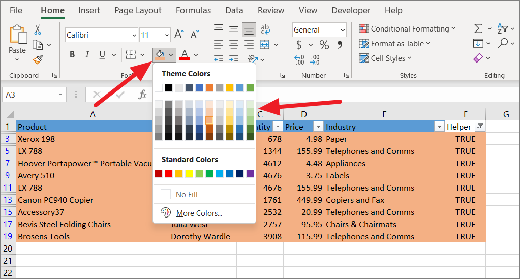
Then, highlight the selected rows with a fill color of your choice.
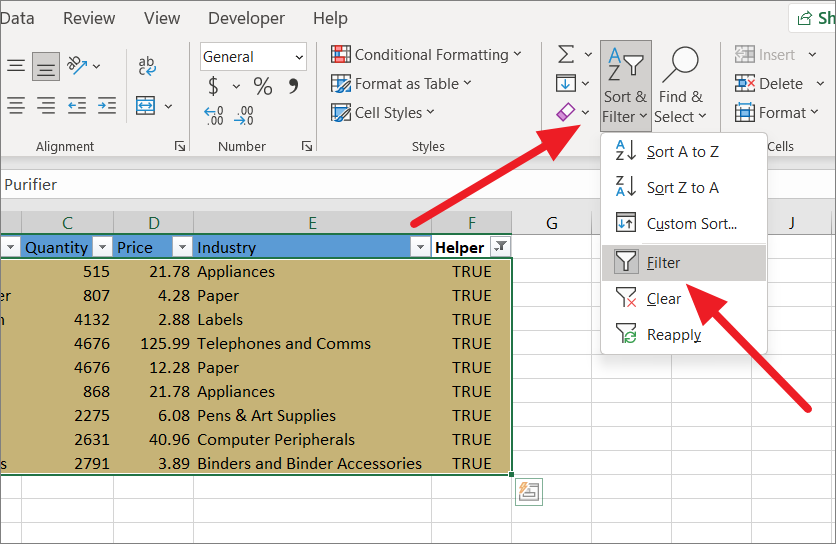
Next, click anywhere in the table or select the entire table, click the ‘Sort & Filter’ button again and select click the ‘Filter’ option to remove the filtering.
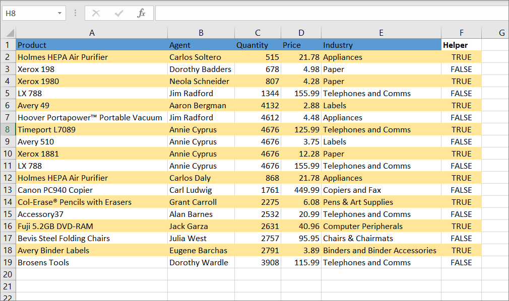
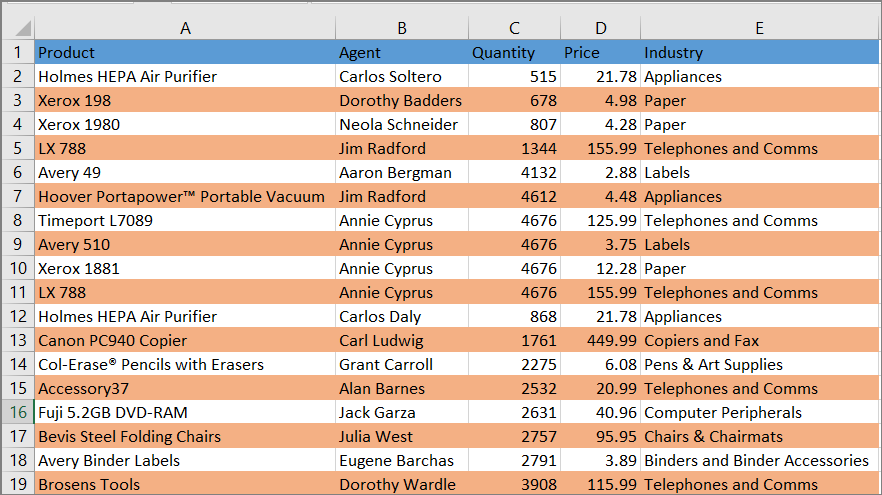
This will expand the table back to the original state and show you that only the alternate even rows are highlighted.
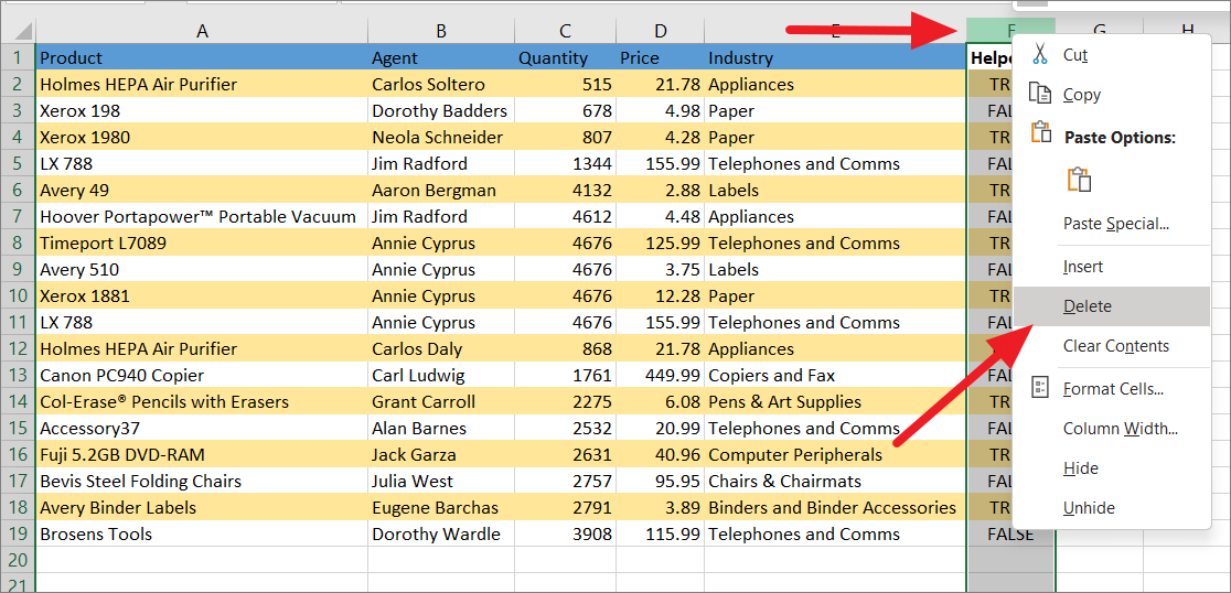
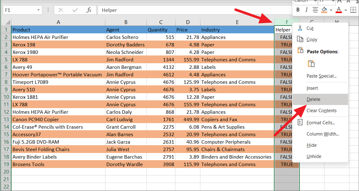
After highlighting the alternate rows, select the Helper column and delete it. If you use the Delete key, it will remove the contents and leave the color shading behind. So, you need to right-click the column header letter (F) and select ‘Delete’.
Result:
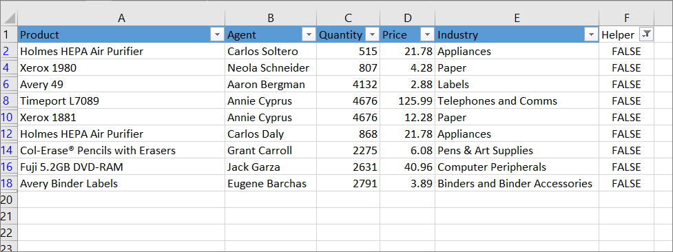
To highlight odd-numbered alternate rows, click the little arrow on the Helper column, uncheck the ‘Select All’ checkbox, and check the ‘FALSE’ option instead. Then, click ‘OK’ to filter the FALSE values.
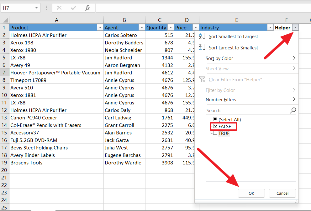
Now, all the column values will be filtered where only the rows with FALSE value (alternate odd rows) will remain visible while others will be hidden.
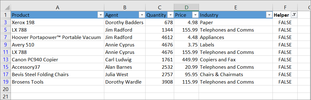
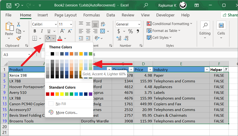
Just like before, highlight the selected rows with a fill color of your choice.
Next, click anywhere in the table or select the entire table, click the ‘Sort & Filter’ button again and click the ‘Filter’ option to remove the filtering.
This will remove the filter, unhide all the rows, and show you that only the alternate odd rows are highlighted.
After highlighting the alternate rows, select the Helper column and delete the entire column.
Highlight Every Other Row using Filter with ISODD and ROW functions.
Similar to the ISEVEN and ROW functions, you can also use ISODD and ROW functions to shade alternate rows in Excel. Similar to the previous method, you can also use the ISODD function to highlight both even-numbered and odd-numbered rows in Excel. ISODD function returns TRUE if the row number is odd. Follow these steps:
First, create a helper column and enter the below formula in the first cell:
=ISODD(ROW())In the above formula, the ROW function returns the row number of the cell, and then the ISODD function returns TRUE if the row number is odd, or else it returns TRUE. Then, click the fill handle and drag your mouse down to autofill the formula for the rest of the cells.
Then, select the range of cells (including the header column) where you want to apply the filter, switch to the ‘Data’ tab, and click the ‘Filter’ button from the ‘Sort & Filter’ group.
Now, all the column values will be filtered by the TRUE value. Then, click the filter button (little arrow button) in the helper column and check the TRUE option and uncheck the FALSE option in the filter options.
Here, if you want to highlighter every other odd row, select the ‘TRUE’ option and deselect the other. Or, if you want to highlight every other even row, select the ‘FALSE’ and deselect the other. Then, click ‘OK’ to filter the column.
Now, all the column values will be filtered. Based on whether you selected TRUE (ODD rows) or FALSE (EVEN rows) in the filter options, either only the odd rows or even rows will be visible respectively.
or
Then, select all the visible rows and highlight them with your desired color.
After that, select the whole table and remove the filtering by switching to the ‘Data’ tab and clicking the ‘Filter’ button or by pressing Ctrl+Shift+L.
Then, select the whole helper column by clicking the column letter (F) and then right-click and select ‘Delete’ to delete it.
Now, you got your odd-numbered rows highlighted in the table below.
You can follow the same instructions and filter the helper column by FALSE value to highlight every other even-numbered row.
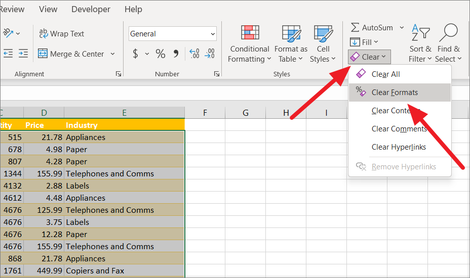
If you don’t want the rows to be highlighted anymore, select the table or the range and click the ‘Clear’ button in the Editing group of the ‘Home’ tab. Then, select ‘Clear Formats’ to remove all formatting from the range.
The result:
Using Conditional Formatting to Highlight Every Other Row in Excel
Excel’s Conditional Formatting is one of the best ways to highlight every other row in a data set because it offers more freedom when applying different formatting to specific rows or columns.
Conditional Formatting allows you to apply formatting to a cell or a range of cells based on the formatting rule. So you can create a conditional formatting rule that uses a formula to find out whether a row is even or odd-numbered and then applies specific formatting based on that.
In Conditional Formatting, you can use two different formulas to shade alternate rows: ISEVEN/ISODD and MOD formulas. However, both formulas need to be created with a conjunction of a ROW function.
Highlight Alternate Even Rows using ISEVEN Function
You can use a formula made up of ISEVEN and ROW functions to highlight or shade colors for the even-numbered rows in a dataset. Here’s how:
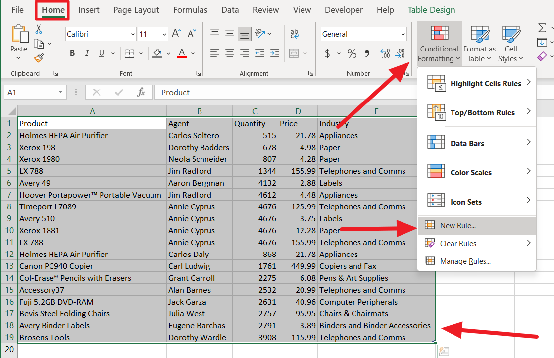
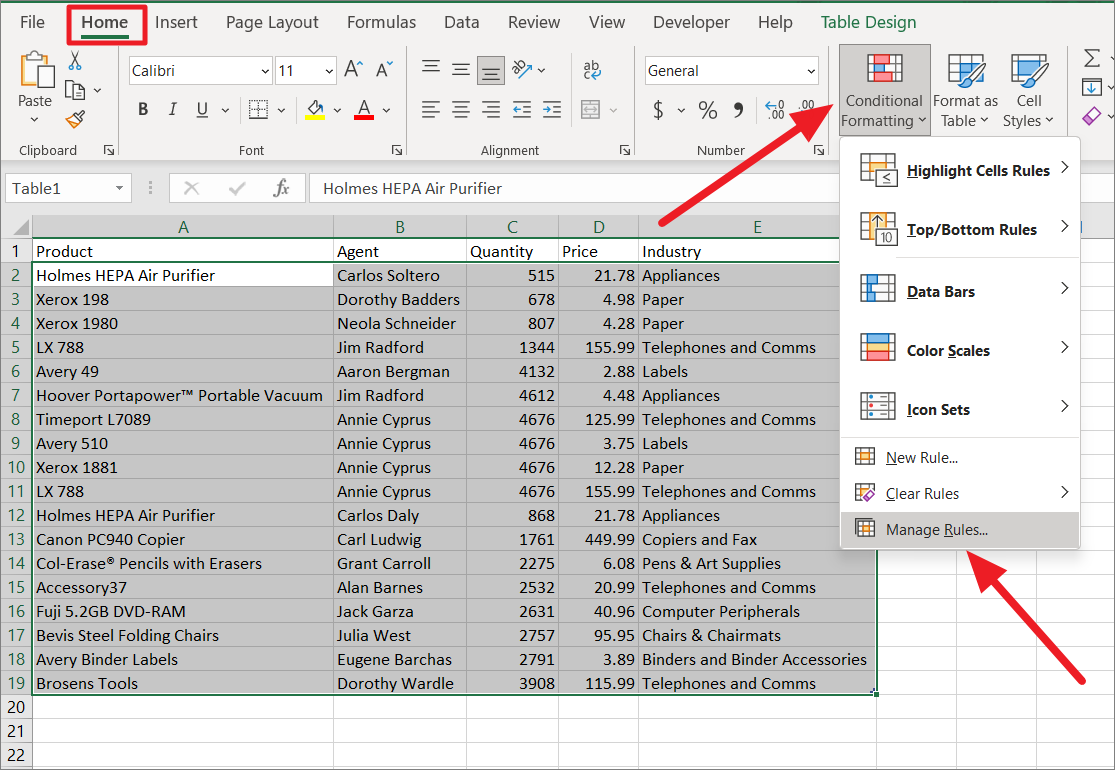
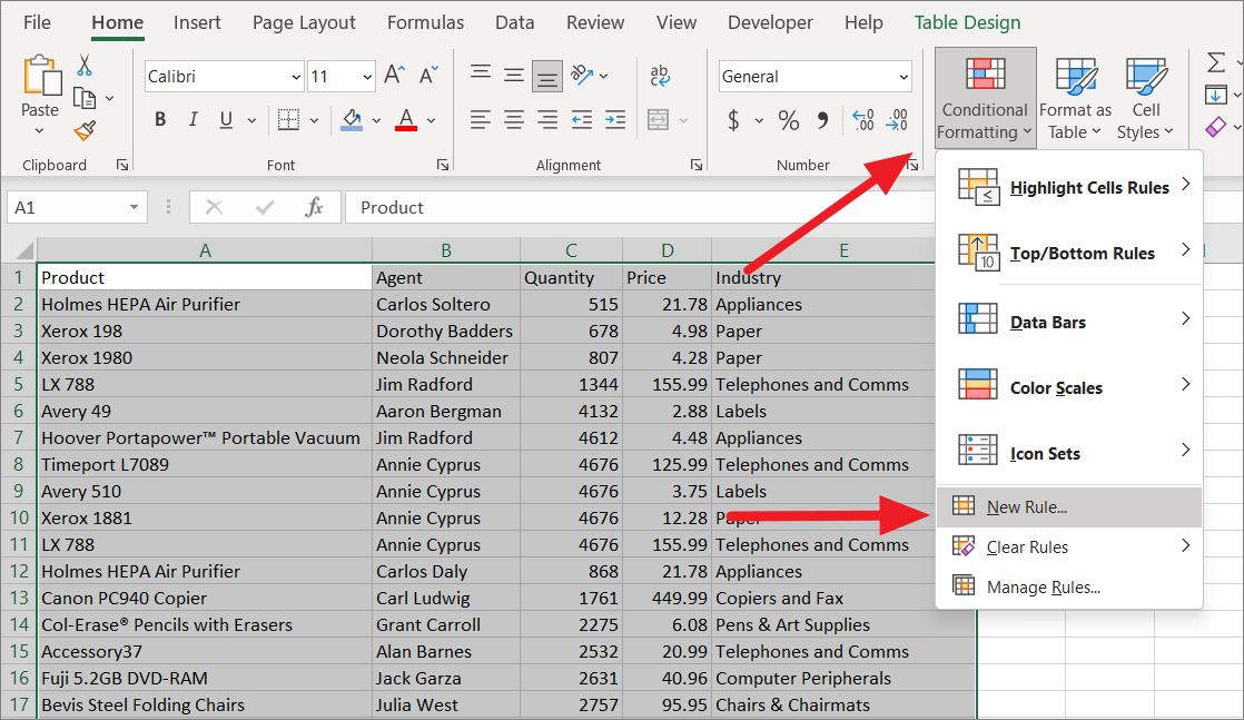
First, select the dataset where you want to highlight. Then, from the ‘Home’ tab, click the ‘Conditional Formatting’ button in the Styles section. From the drop-down menu, select the ‘New Rule…’ option.
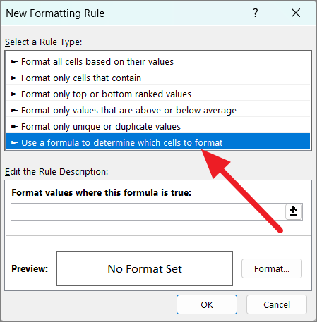
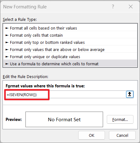
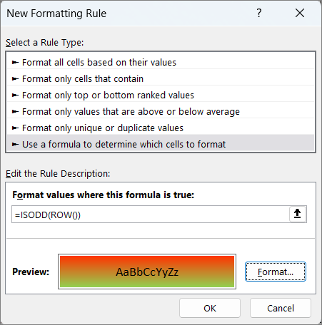
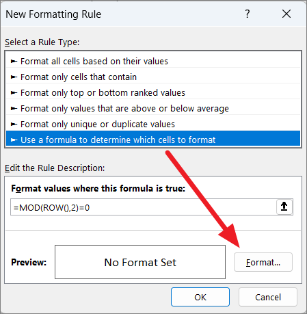
This will launch the New Formatting Rule dialog window. Here, select the ‘Use a formula to determine which cells to format’ option under the ‘Select a Rule Type’ section. This will open up a box below where you can enter the formula and specify formatting.
Now, type the below formula in the input field under the ‘Edit the Rule Description:’ section.
=ISEVEN(ROW())In the above formula, the nested ROW function returns the row number, and then the ISEVEN function checks whether that number is even or not. The formula determines whether the row is even-numbered or not and returns TRUE. If the condition is TRUE, then specific formatting is applied to the row.
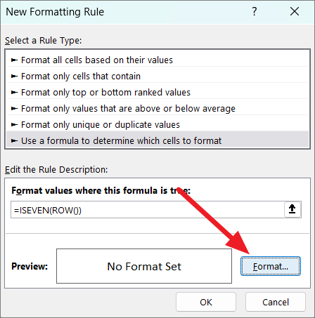
Next, click the ‘Format’ button below to specify the formatting you want to use highlight the alternate rows.
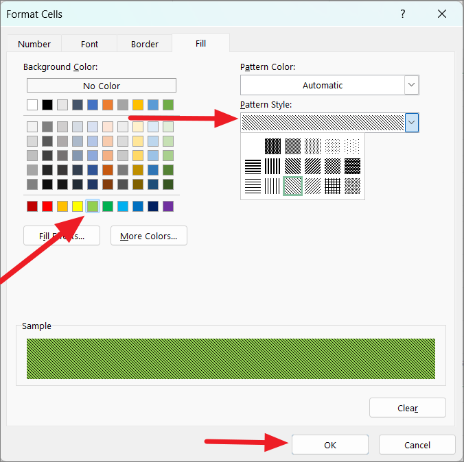
In the Format Cells dialog box, switch to the ‘Fill’ tab and choose the color for highlighting. You can choose a pattern style for the fill color from the ‘Pattern Style’ drop-down. Then, click ‘OK’.
If you made mistakes while selecting format, you can always click the ‘Clear’ button to remove the formatting.
In the New Formatting Rule dialog box, you can see a preview of what each highlighted cell would look like. Now, click ‘OK’ to apply the conditional format.
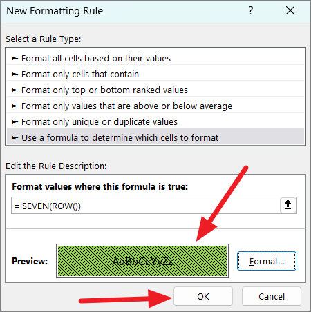
The Conditional Formatting rule will check each row against the given formula and if a row meets the condition (returns TRUE), it will highlight that row with the specified format.
Now, all the alternate rows of your dataset will be highlighted with the selected formatting.
Highlight Alternate ODD Rows using ISODD Function
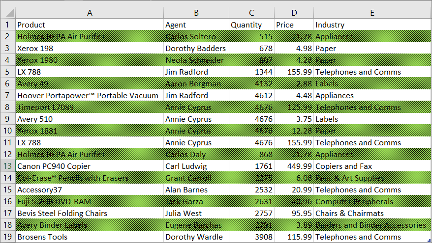
Similarly, you can use the ISODD and ROW functions to highlight or shade colors for the odd-numbered rows in a dataset.
First, select the dataset where you want to highlight. Then, from the ‘Home’ tab, click the ‘Conditional Formatting’ button in the Styles section. From the drop-down menu, select the ‘New Rule…’ option.
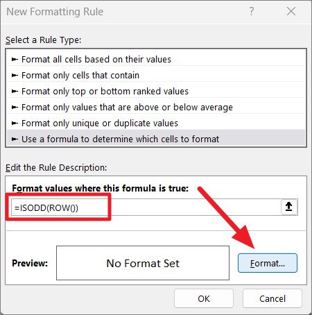
This will launch the New Formatting Rule dialog window. Here, select the ‘Use a formula to determine which cells to format’ option under the ‘Select a Rule Type’ section. This will open up a box below where you can enter the formula and specify formatting.
Now, type the below formula in the input field under the ‘Edit the Rule Description:’ section.
=ISODD(ROW())The above formula is used to determine whether the row is even-numbered or not. Next, click the ‘Format’ button below to specify the formatting you want to use highlight the alternate rows.
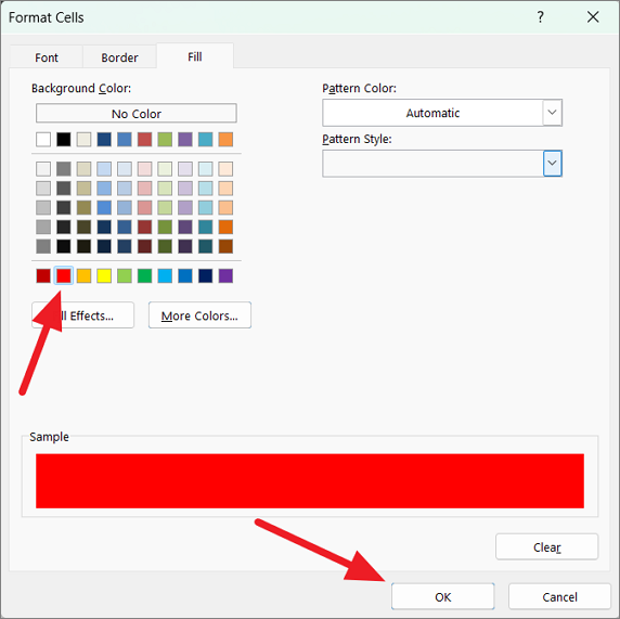
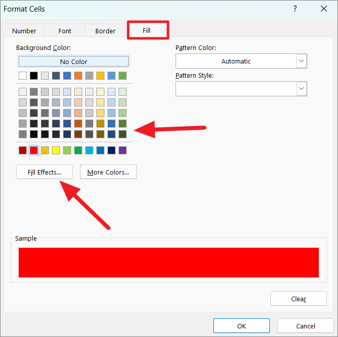
In the Format Cells dialog box, switch to the ‘Fill’ tab and choose the color for highlighting. To make your row highlights a little more attractive, you can add gradient effects. To add gradient effects, click the ‘Fill Effects…’ button.
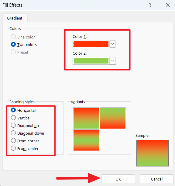
This will open another window named Fill Effects where you choose your gradient effects. Here, first, choose colors from the color drop-down. You can either select one color or two colors from the dropdowns. Here, we selected the red color from the ‘Color 1’ drop-down and the green color from the ‘Color 2’ drop-down.
Then, select a shading style and one of their variants. After selecting the gradient effects, click ‘OK’ twice.
Once the formatting is selected, click ‘OK’ in the New Formatting Rule dialog box.
Now, all the alternate rows of your dataset will be highlighted with the selected formatting.
Highlight Both Even and ODD Rows using ISEVEN and ISODD functions
In case you want to highlight even rows in one color and odd rows in another color, you can do that by creating two conditional formatting rules with ISEVEN and ISODD functions and applying both rules to the same range. Here’s how you can do that:
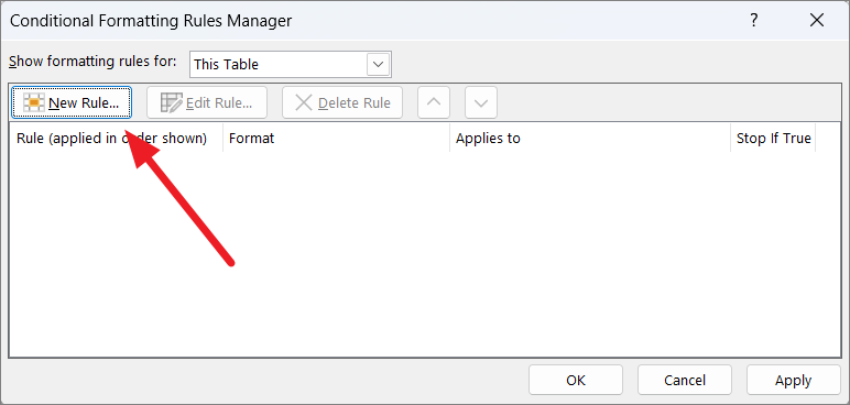
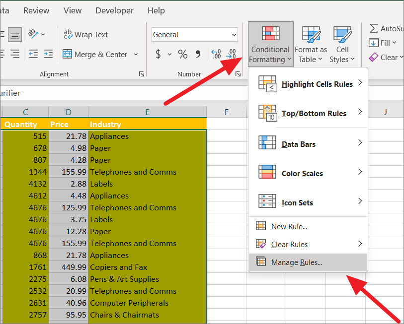
First, select the dataset and then open the Conditional Formatting Rules Manager by clicking the ‘Conditional Formatting’ menu in the ‘Home’ tab and selecting ‘Manage Rules…’.
This will open up the Conditional Formatting Rules Manager window. If you already applied a formatting rule based on ISEVEN() or ISODD() function, or any other rule, it will be listed in the Rule box. In that case, you just have to add a second rule.
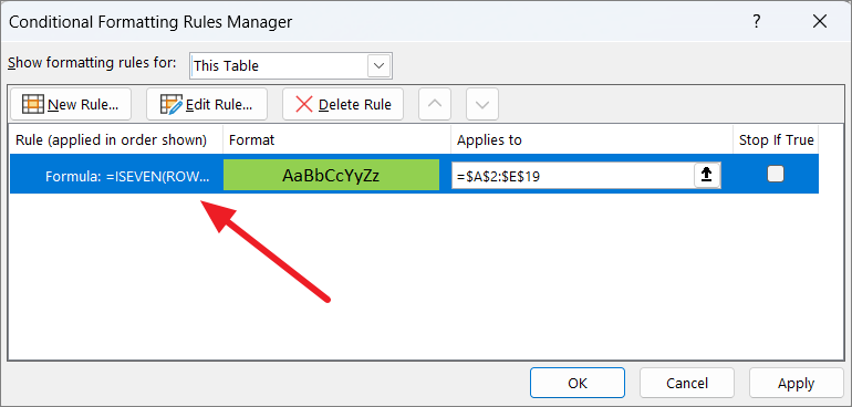
If not, you have to add two conditional formatting rules one for ISEVEN and another for ISODD. To do that, click the ‘New Rule…’ button.
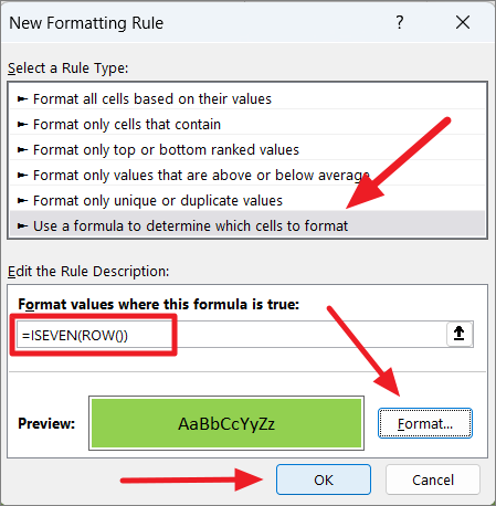
Then, select the ‘Use a formula to determine which cells to format’ option from the ‘Select a Rule Type:’ box and below formula in the input field below:
=ISEVEN(ROW())After entering the formula, use the ‘Format’ option to specify the formatting you want to apply to the even rows just like we did in the previous method. Then, click ‘OK’ to save the rule and get back to the Conditional Formatting Rules Manager.
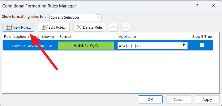
Next, click the ‘New Rule…’ button again to add another rule for odd rows.
Now follow the same instructions, enter the below formula in the Edit the Rule Description box, specify the formatting for odd rows, and click the ‘OK’.
=ISODD(ROW())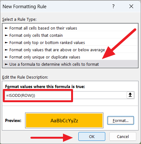
After creating both rules, click ‘Apply’ and then ‘OK’.
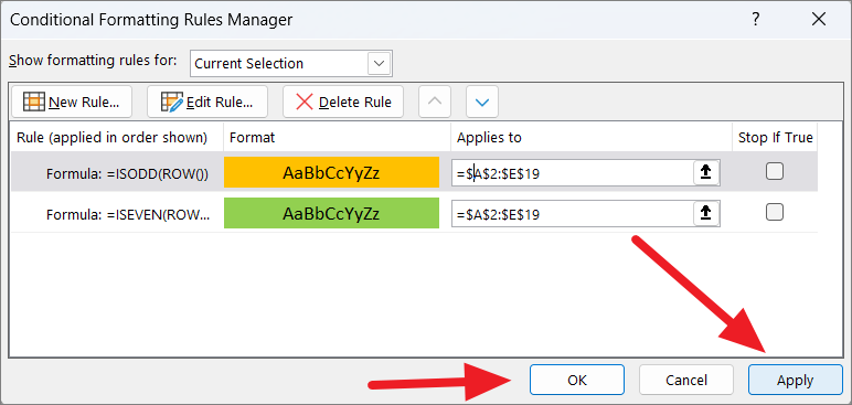
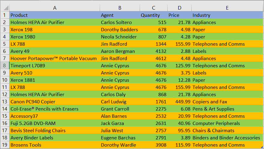
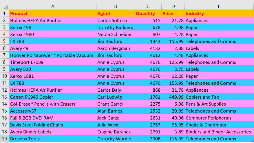
This will apply unique color shading for every other even row and odd row based on two colors.
Highlight Alternate Rows using the MOD function
Another formula that can be used to highlight every other row is based on the combination of MOD and ROW functions which are more flexible than the ISODD and ISEVEN functions. Plus, if you are using an Excel version lower than 2007, ISEVEN and ISODD may not be available in that version. The MOD function is used to return the remainder after division. Follow these steps to highlight alternate rows using the MOD function with conditional formatting.
Select the dataset where you want to shade rows. From the ‘Home’ tab, click the ‘Conditional Formatting’ menu in the Styles section, and select the ‘New Rule’ option.
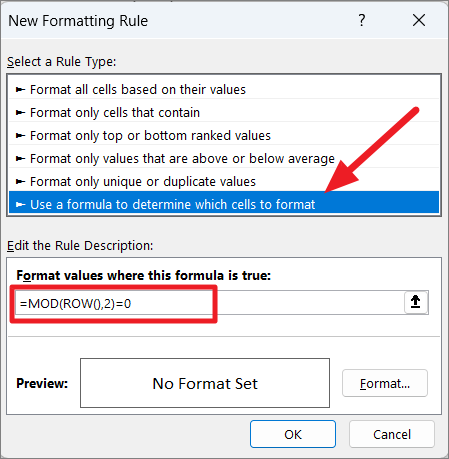
In the New Formatting Rule window, select ‘Use a formula to determine which cells to format’ from the Select a Rule Type: section.
To highlight even-numbered alternate rows, enter the below formula in the formula field:
=MOD(ROW(),2)=0Explanation:
- In the formula, the MOD function takes two arguments – number (which is provided by the ROW function) and the divisor (which is set as 2) and returns a reminder.
- As we have seen before, the ROW function returns the row number of the active cell. If the remainder of a division (the result of MOD) is equal to ‘0’, the formula returns TRUE. So, if the result of the formula is TRUE, the specified formatting will be applied to that row.
- The formula starts checking from the first row of the selected range. For example, the first row number is 1 (returned by ROW) which is divided by 2 and returned 1 as a remainder. If row number 2 is divided by 2, it returns 0 as a remainder, and so on. If the row number is odd, the MOD function always returns 1 as remainder and if the row number is even, it returns 0.
- So, the MOD function produces ‘0’ for all even-numbered rows (2, 4, 6, etc.) which satisfies the condition (=0) of the given formula. As a result, the formula returns TRUE for every even row. Hence, only the even rows are highlighted with the specified format.
Then, click the ‘Format’ button to select the formatting color for highlighting.
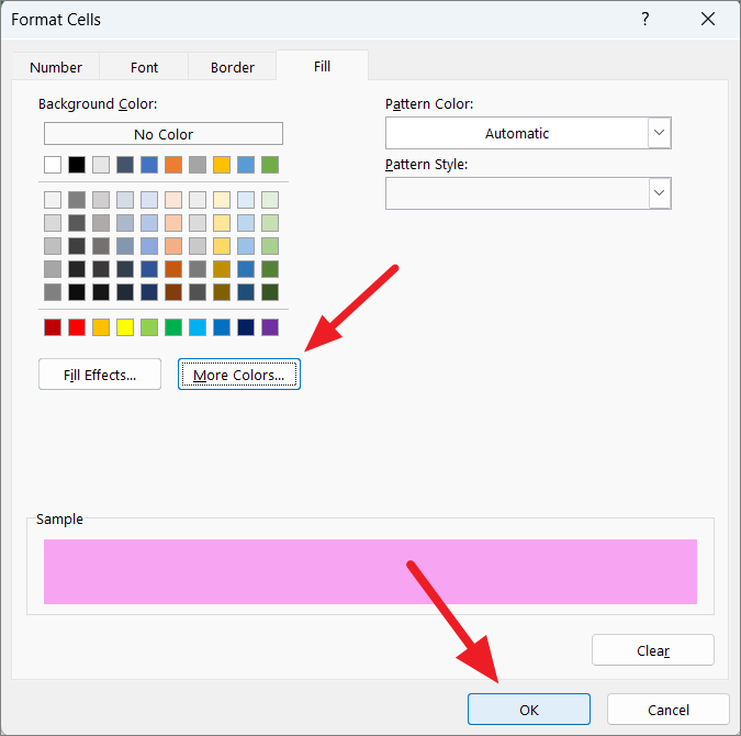
In the Format Cells window, go to the ‘Fill’ tab and pick a color and if you can’t find the color you want in the preset options, select the ‘More Colors…’ button to get more colors. After selecting the color and formatting, click ‘OK’.
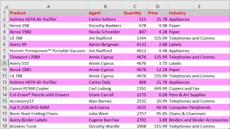
You have highlighted alternate even rows:
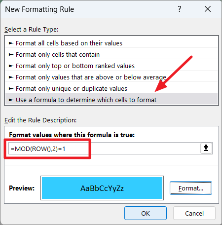
To highlight odd-numbered alternate rows, use this formula instead, in the formula field of the New Formatting Rule window:
=MOD(ROW(),2)=1This formula is similar to the previous formula except the formula result needs to be equal to 1. If the MOD function divides odd numbers (odd row number) by 2, it always returns ‘1’ as a reminder that satisfies the condition (=1), and for even rows, it returns 0. Hence, only the odd rows are formatted by this condition.
Then, specify the formatting using the ‘Format…’. option and click ‘OK’.
This will highlight the odd-numbered alternate rows for you:
Or if you apply both odd and even row formatting rules, you will get the below result:
Highlight Every nth Row with Conditional Formatting
If you want to highlight every 3rd, 4th, or nth row in a table, you can also do that with conditional formatting. You can build a formatting rule based on MOD and ROW functions to shade every nth row in a table.
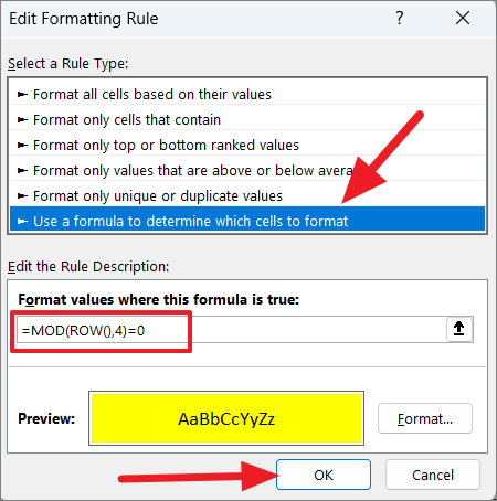
For example, to highlight every 4th row, use the below formula for the formatting rule:
=MOD(ROW(),4)=0Where replace ‘4’ with the nth number of rows you want to highlight.
Here, the divisor is 4, so the MOD function divides each row number by 4 and returns ‘0’ as a remainder only when divided by every 4th-row number (4, 8, 12, etc.). Hence, only rows 4, 8, 12, 16, etc. will be highlighted.
Then, choose a format and click ‘OK’ to apply the conditional formatting.
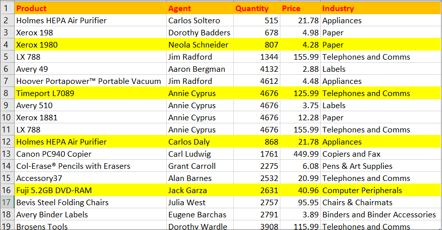
As a result, only every 4th row is shaded with the selected color format.
Highlight Alternate Columns with Conditional Formatting
With Conditional Formatting, you can also shade color for alternate columns in Excel. The formula for highlight columns is similar to the formula for rows except you have to use the MOD function with COLUMN function instead of the ROW function. Here’s how:
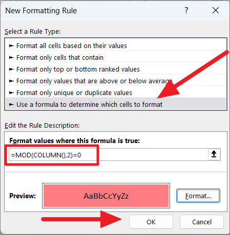
Select the range where you want to alternate column colors, go to the ‘Conditional Formatting’ menu in the Home tab and select ‘New Rule’. Then, select the ‘Use a formula to determine which cells to format’ option and enter the below formula:
=MOD(COLUMN(),2)=0The nested COLUMN function finds and returns the column numbers which is then used as the number argument of the MOD function. The MOD function divides the column number by 2 and returns ‘0’ as a reminder for every even-numbered column. If the condition is TRUE, the alternate even rows get highlighted.
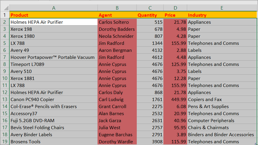
As you can see, every alternate even-numbered column is highlighted.
To highlight odd-numbered columns, use this formula instead:
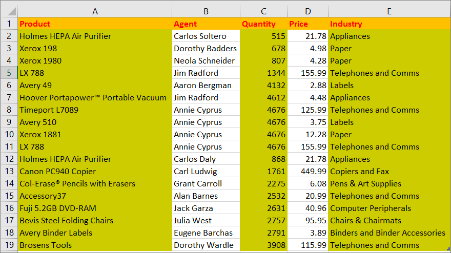
=MOD(COLUMN(),2)=1The result:
Edit Conditional Formatting Rule
Another advantage of using the Conditional formatting method is that you can edit the formatting rule at any time to make changes to your highlight. For instance, if you already highlighted even rows in your table, you can easily edit the formula in the formatting rule to highlight odd rows. Here’s how you can do that:
Select the range where conditional formatting is applied, click the ‘Conditional Formatting’ menu, and select ‘Mange Rules..’.
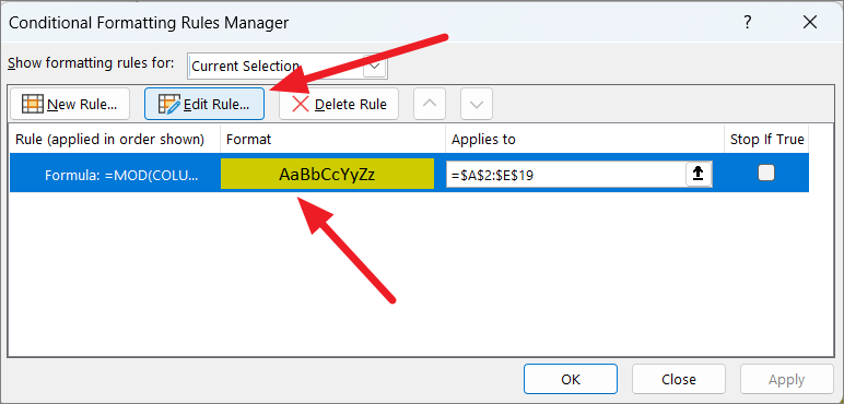
When the Conditional Formatting Rules Manager launches, select the rule you want to change and click the ‘Edit Rule…’ button to edit the formula, formatting, etc.
Remove Row Highlights
If you no longer want your rows to be highlighted, you can clear or delete rules to remove highlights. To do that, follow these steps:
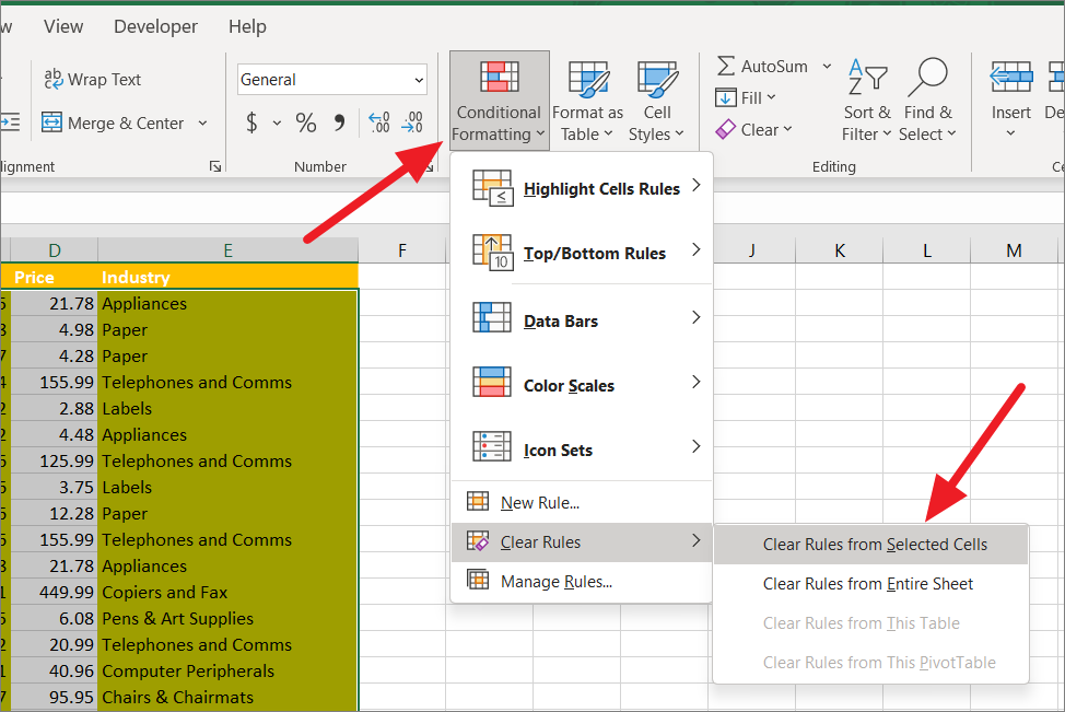
Select the data range where rows are highlighted with conditional formatting, click the Conditional Formatting menu, and hover over ‘Clear Rules’. And then select ‘Clear Rules from Selected Cells’ or ‘Clear Rules from Entire Sheet’ from the submenu.
To remove a specific formatting rule, select the ‘Manage Rules’ option from the ‘Conditional Formatting’ menu.

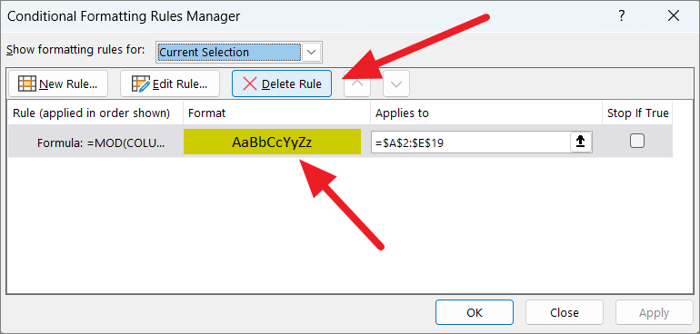
Then, select a specific rule from the Rule Manager and click ‘Delete Rule’ to remove the formatting.
Hopefully, this article helps you highlight every other row and column in Excel to make your worksheets readable and user-friendly.


