How to Insert a Drop Down Menu in Google Sheets

A drop-down list, also referred to as a drop-down menu or pulldown menu, allows users to select an option from a predefined set of choices. This feature ensures that only specified values are entered into cells, reducing errors and streamlining data entry.

When collaborating on Google Sheets, there may be instances where you need others to input consistent values in a specific column. To minimize inaccuracies and typing errors, adding a drop-down list can enforce the use of predetermined options.

For instance, if you’re managing a list of tasks for your team and want members to update the status of each task with options like Done, Pending, Priority, Skipped, or Task-in progress, a drop-down menu can simplify this process by providing these options directly.

This guide delves into creating and managing drop-down lists in Google Sheets, offering detailed steps to enhance your spreadsheets.

Creating a Drop-Down List in Google Sheets

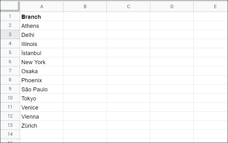
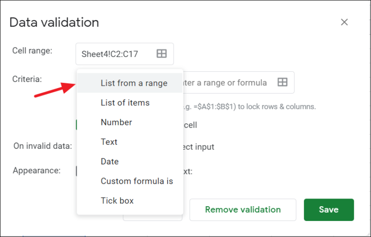
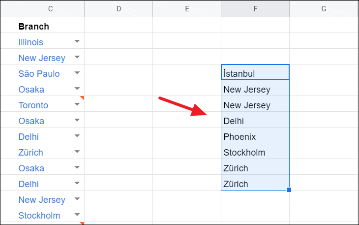
The drop-down feature in Google Sheets utilizes data validation to control the inputs allowed in your worksheet. You can create a drop-down list either by using a range of cells containing your options or by manually specifying the items.

Using a Range of Cells for Your Drop-Down Menu

To create a drop-down list based on a range of cells:

Open your Google Sheets document and enter the list of items you want to include in your drop-down menu. In this example, we’ve listed city names as branch locations.

Select the cell or range of cells where you want the drop-down menu to appear. This can be on the same sheet or a different one.

Click on the Data menu at the top and choose Data validation from the drop-down options.

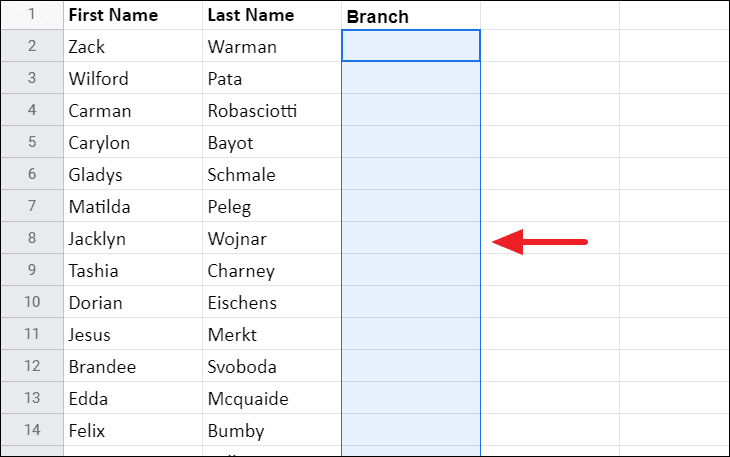
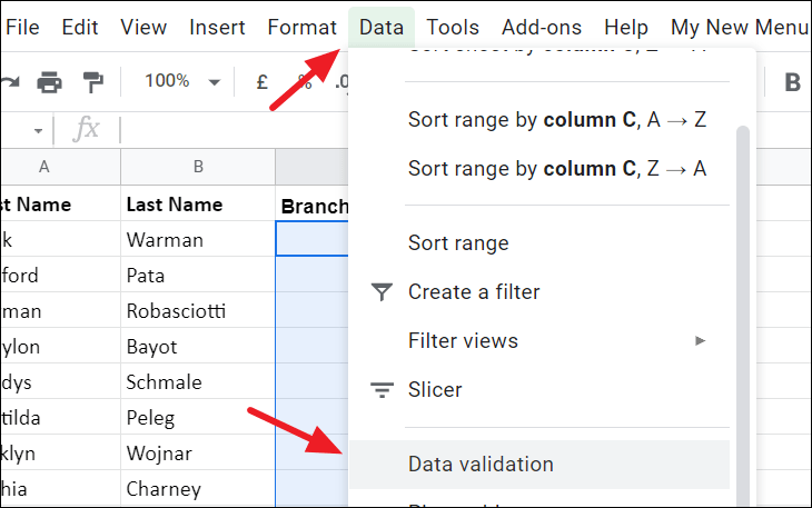
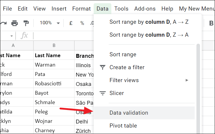
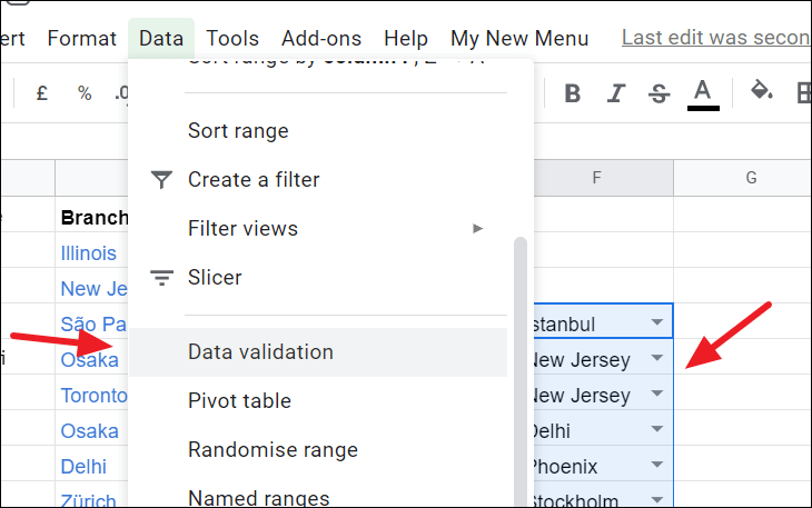
You can also right-click on the selected cells and choose Data validation from the context menu.

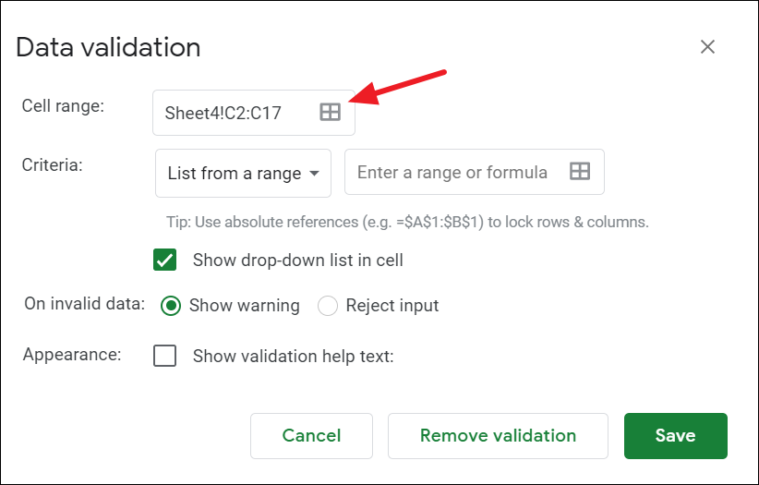
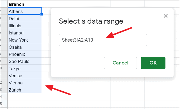
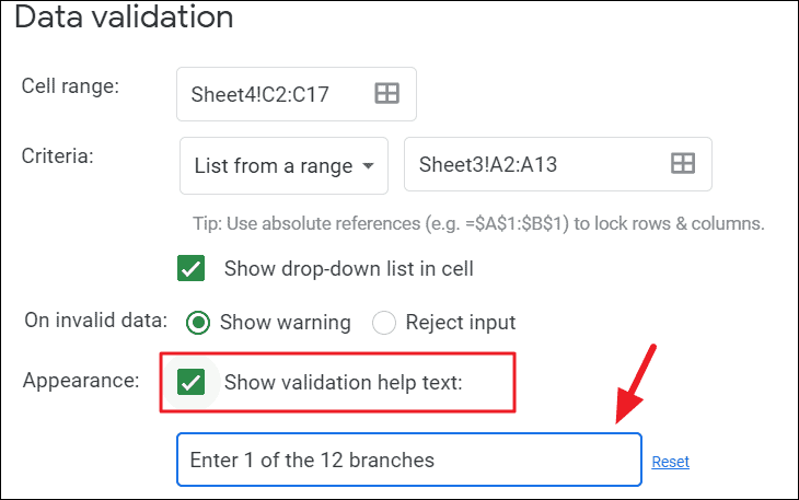
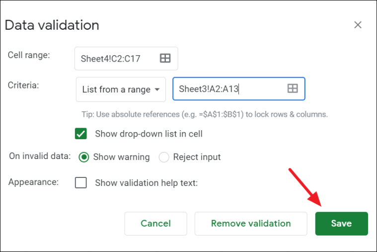
In the Data validation dialog box, you’ll see several settings to customize your drop-down list.

The Cell range field will display the cells you’ve selected for the drop-down list. You can adjust this by clicking the grid icon and selecting a different range if needed.

Under Criteria, select List from a range from the drop-down menu. In the field next to it, enter the range of cells containing your list items. Click the grid icon to easily select the range on your sheet.

In the Select a data range dialog, choose the cells with your list items. The selected range will appear in the field. Click OK to confirm.

Ensure that the Show dropdown list in cell option is checked. This displays the drop-down arrow in the cell for users to access the list.

Decide how to handle invalid data entries under On invalid data. Choose Show warning to accept the input with a warning, or Reject input to prevent any entries not on the list.

In the Appearance section, you can provide a helpful message for users. Check Show validation help text and enter your instructions in the text box that appears.

Click Save to apply your settings and create the drop-down list.

Understanding How the Drop-Down List Works

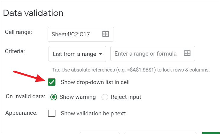
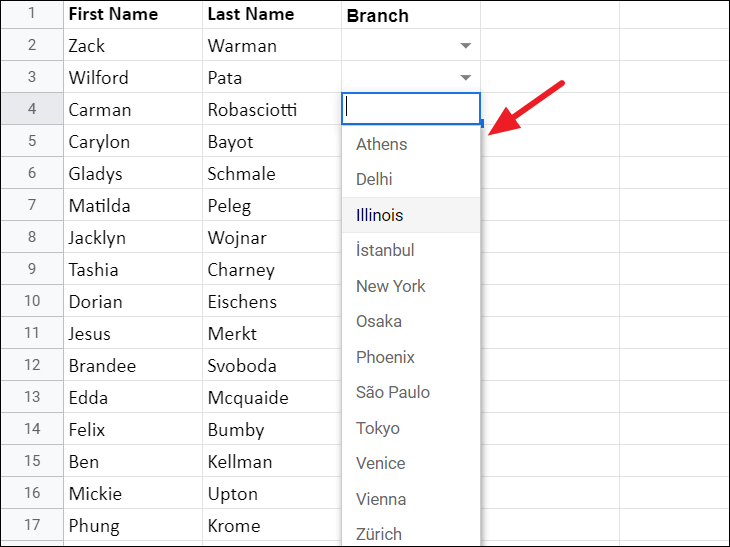
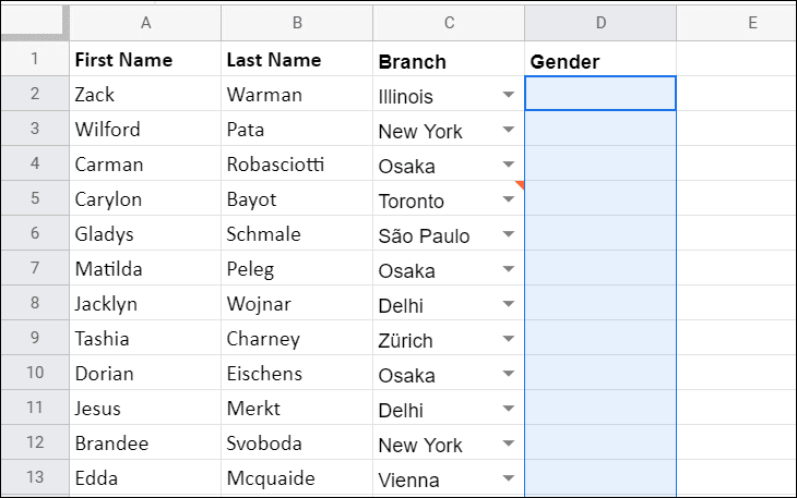
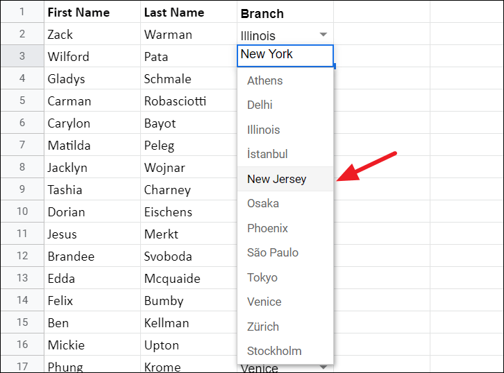
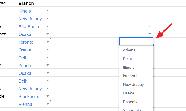
With the drop-down list now in place, clicking the drop-down arrow in cells C2:C17 will display your list of items.

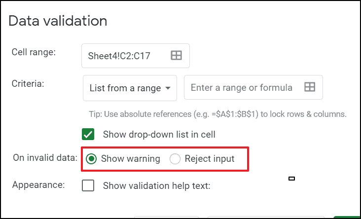
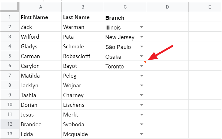
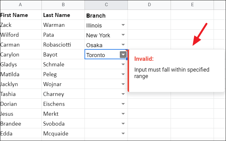
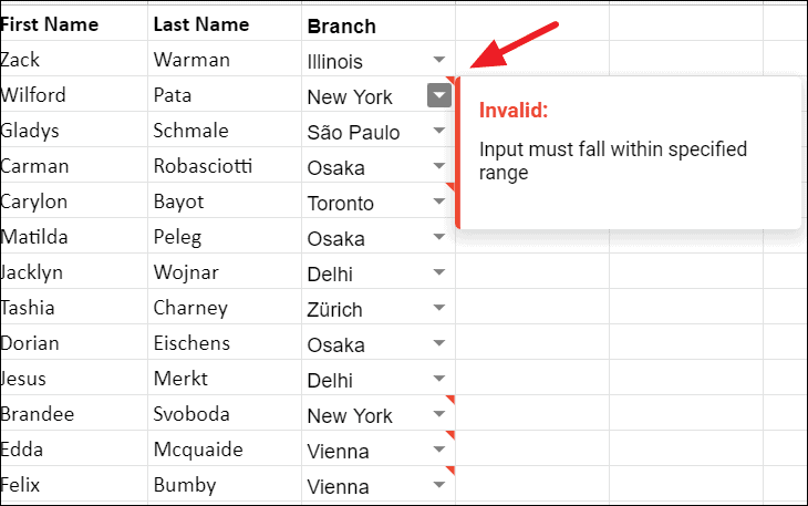
If a user enters a value not included in the list and you’ve selected Show warning, the cell will be marked to indicate invalid data. For example, notice the marker in cell C6 indicating such an entry.

Hovering over the marker will display a warning message, alerting the user to the invalid entry.

This method allows you to create dynamic drop-down lists that reference cell ranges, ensuring your list stays updated with any changes to the source data.

Manually Entering Items for Your Drop-Down Menu

If you prefer to create a static drop-down list without sourcing items from a cell range, you can manually enter the options directly:

Select the cell or cells where you want to add the drop-down menu.

Go to the Data menu and select Data validation.

Ensure the correct cell range is specified. In the Criteria section, select List of items from the drop-down menu.

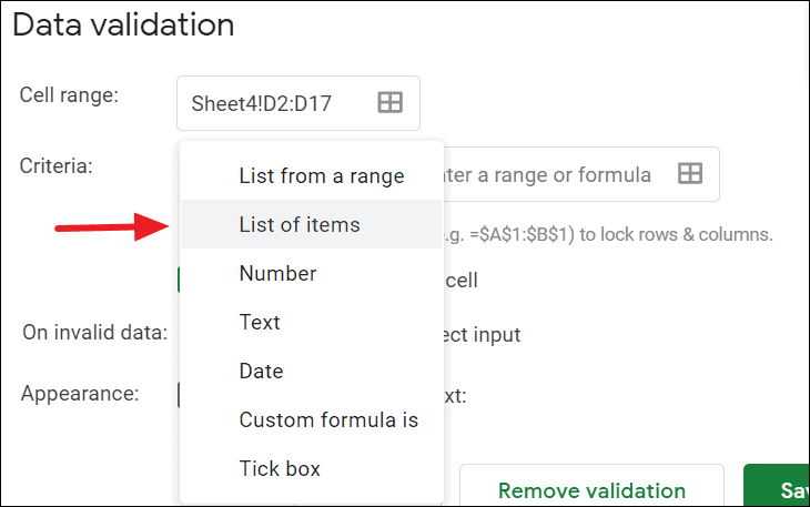
In the field provided, type your list items separated by commas without spaces. For example, enter Male,Female,Not Specified to create a gender selection list.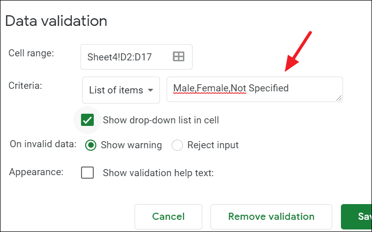

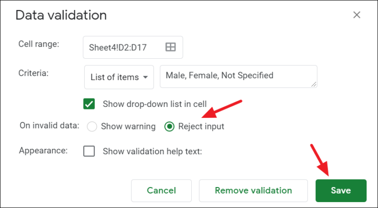
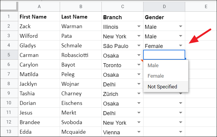
Check the Show dropdown list in cell option. Under On invalid data, select Reject input to prevent users from entering values outside your specified items.

Click Save to create the drop-down list.

Now, each selected cell will contain a drop-down menu with your specified items. Users can click the drop-down arrow or press Enter to select an option.

If a user attempts to enter an invalid value, the input will be rejected, and an error message will prompt them to select a valid option.

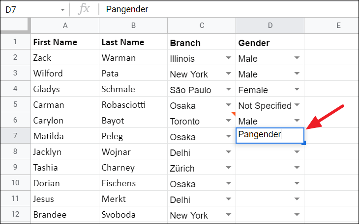
The error message will inform the user of the invalid entry and guide them to enter one of the specified values.

Editing a Drop-Down List in Google Sheets

There might be occasions when you need to update your drop-down list by adding, changing, or removing items. Here’s how to modify your existing drop-down lists:

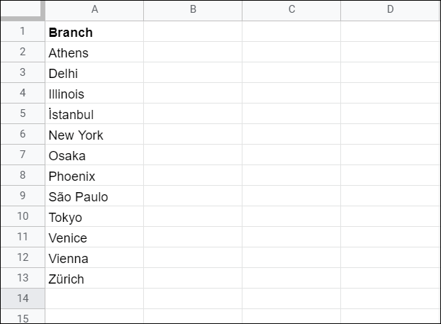
Navigate to the range of cells containing the source list for your drop-down menu. Make the necessary changes, such as adding new items, editing existing ones, or deleting items.

Original list:

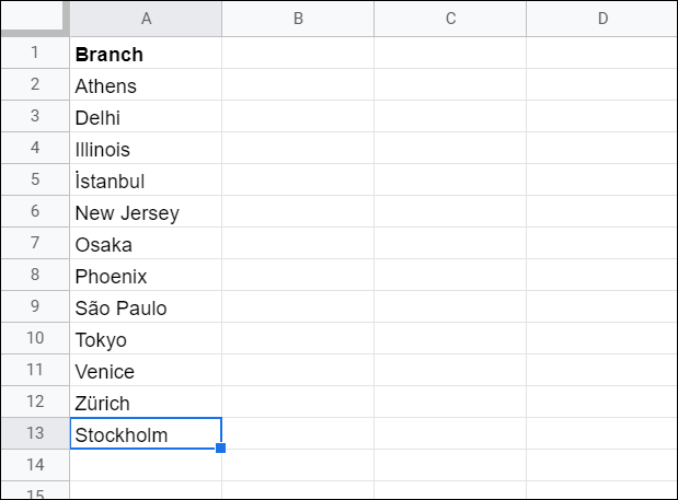
Updated list with changes:

If you manually entered items when creating the drop-down list, you can edit them directly in the Data validation dialog box.

After updating the source list, your drop-down menu will automatically reflect these changes. However, any previously selected items that no longer exist in the updated list will be marked as invalid.

Click on the drop-down arrow to view and select from the updated list of items.

Note: If you’ve added or removed items and expanded or reduced your list’s range, make sure to update the range in the Data validation settings accordingly.

Copying a Drop-Down List in Google Sheets

To apply the same drop-down list to multiple cells or sheets without recreating it each time, you can copy and paste the drop-down list:

Select the cell containing the drop-down list and copy it by right-clicking and choosing Copy or pressing Ctrl + C.

Select the target cell or range where you want to duplicate the drop-down list.

Right-click on the selected cells, expand Paste special, and choose Paste data validation only.

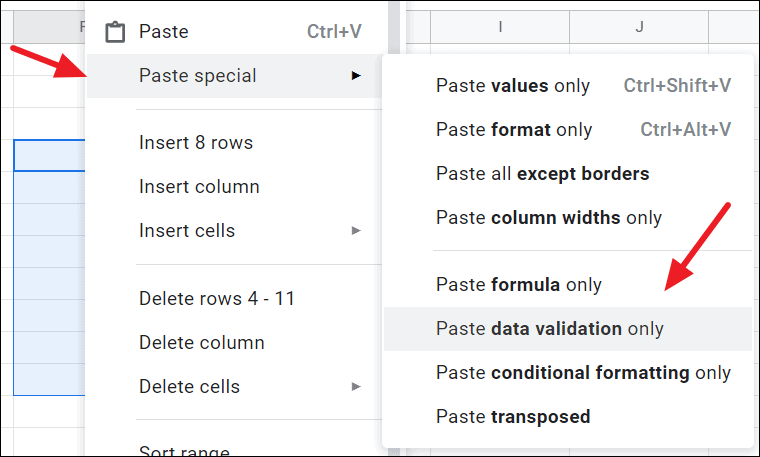
This method copies only the drop-down list without altering any existing cell formatting or content.

Removing a Drop-Down List in Google Sheets

If you no longer need a drop-down menu in your spreadsheet, you can remove it easily:

Select the cell or range of cells containing the drop-down list you wish to delete.

Go to the Data menu and select Data validation.

In the Data validation dialog box, click on the Remove validation button at the bottom.

Click Save to confirm and remove the drop-down list from the selected cells.

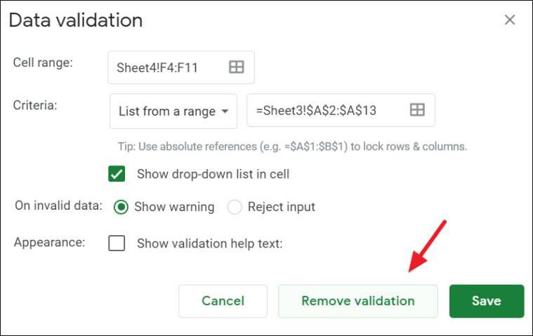
The drop-down menu will be removed, but any data previously entered using the drop-down list will remain in the cells.

By utilizing drop-down lists in Google Sheets, you can ensure data consistency and accuracy across your spreadsheets. Whether you’re collecting specific information or streamlining data entry, drop-down menus are a valuable tool for effective spreadsheet management.