Excel provides powerful tools to help you organize and arrange your data effectively, allowing for quick retrieval and analysis. You can sort data based on text, numbers, dates, times, and even cell colors or custom icons. This guide will walk you through various methods to sort data in Excel, ensuring your information is structured exactly as you need it.

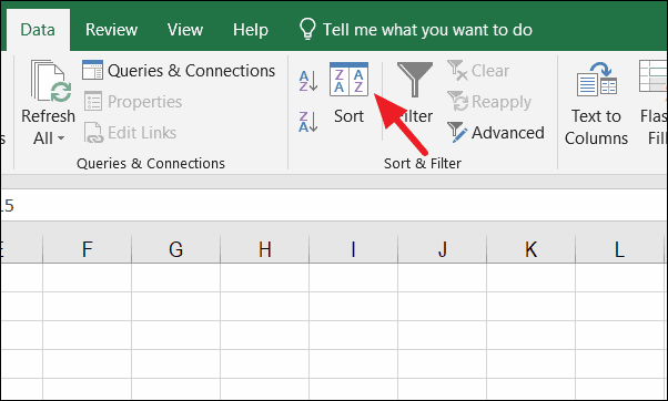
Sorting data in Excel

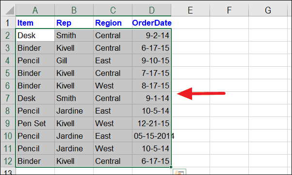
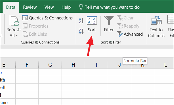
Before you begin sorting, decide whether you want to rearrange the entire worksheet or just a specific range of cells. Sorting can be applied to one column, multiple columns, or only a portion of your data without affecting the rest of the worksheet.

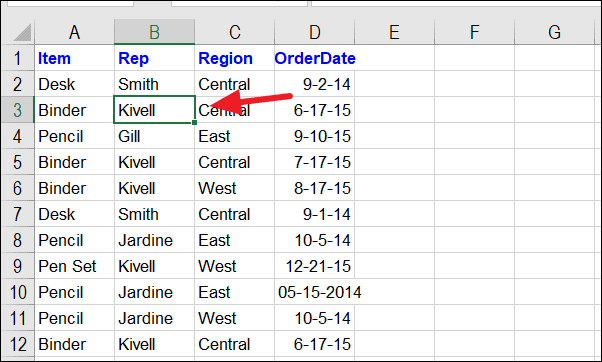
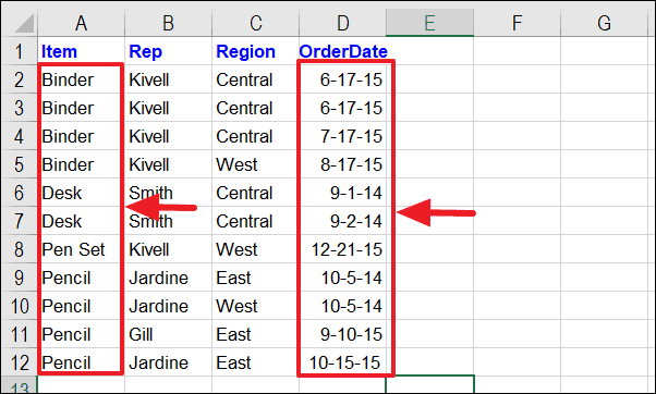
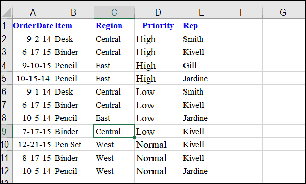
For example, suppose you have the following dataset and you want to sort the data based on the representatives’ names.

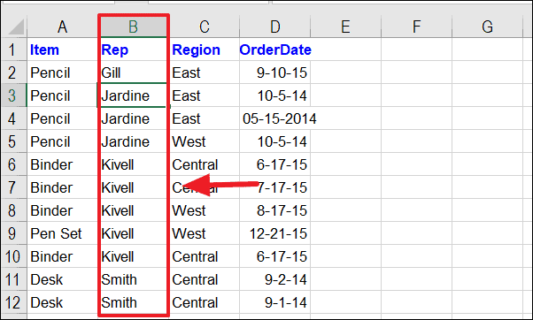
Click on any cell within the column you wish to sort. In this case, click on any cell in column B, which contains the ‘Rep’ names.

Navigate to the Data tab on the Excel ribbon and click on the ‘A to Z’ sort icon to sort the data alphabetically by the selected column.

After performing the sort, your dataset will be rearranged so that the representatives’ names are in alphabetical order, and all corresponding data in each row moves along with them.

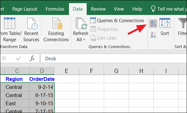
Sorting data by date or time

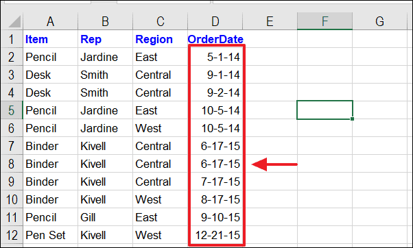
Excel allows you to sort data based on dates and times, arranging them from oldest to newest or vice versa. This is particularly useful when you’re dealing with time-sensitive information.

Click on any cell within the column containing the dates or times you wish to sort. For instance, select a cell in the ‘OrderDate’ column.

Go to the Data tab and click on the ‘Sort’ icon, which opens the Sort dialog box for more advanced sorting options.

In the Sort dialog box, select ‘OrderDate’ from the ‘Sort by’ dropdown menu. Then, choose ‘Newest to Oldest’ or ‘Oldest to Newest’ from the ‘Order’ dropdown to specify the sorting order.

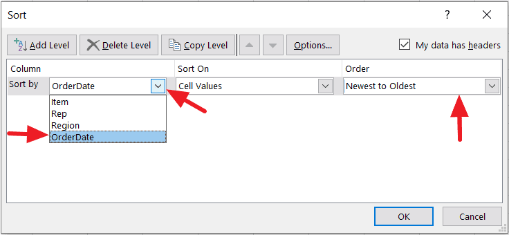
Once you click ‘OK’, your data will be sorted according to the specified date order.

Sorting data by cell color, font color, or cell icon

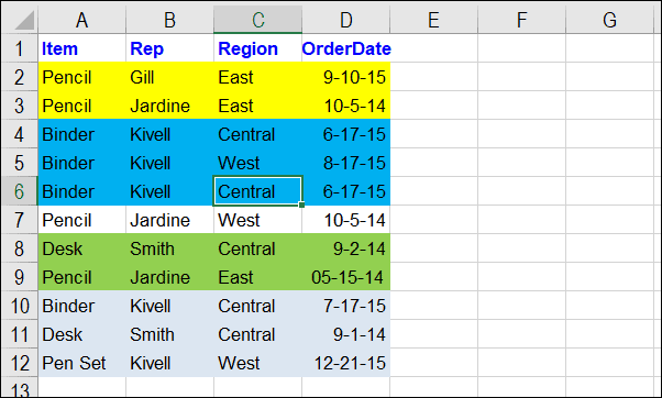
If your data includes cell formatting such as cell colors, font colors, or icons, you can sort based on these attributes to bring certain records to the forefront.

Click anywhere in the data range and open the ‘Sort’ dialog box from the Data tab.

In the Sort dialog box, choose the column you want to sort from the ‘Sort by’ dropdown. Then, select ‘Cell Color’, ‘Font Color’, or ‘Cell Icon’ from the ‘Sort On’ dropdown menu, depending on your needs.

In the ‘Order’ section, select the color, font, or icon you want to sort by, and specify whether it should appear on top or bottom.

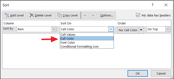
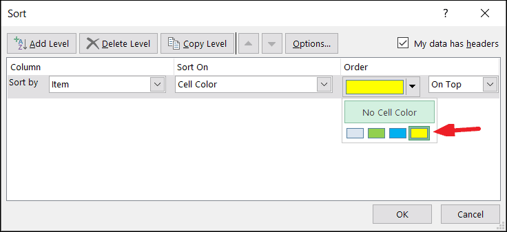
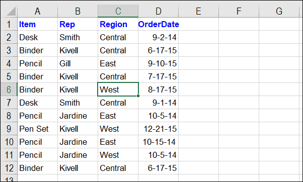
Click ‘OK’ to apply the sort. Your dataset will now be organized based on the specified cell formatting.

Sorting multiple columns (multiple level data sorting)

To sort data by more than one column, you can perform a multi-level sort. This allows you to organize your dataset first by one column and then by another.

Select any cell within your dataset and open the ‘Sort’ dialog box from the Data tab.

In the Sort dialog box, choose the primary column you want to sort by from the ‘Sort by’ dropdown. For example, select ‘Item’.

Click on ‘Add Level’ to add another sorting criterion. Then, select the second column from the ‘Then by’ dropdown, such as ‘OrderDate’. Set the desired sorting order for each column.

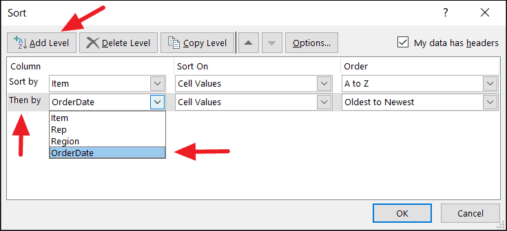
After clicking ‘OK’, your data will be sorted first by ‘Item’ and then by ‘OrderDate’.

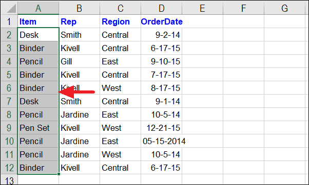
Sorting data in only one column

In some cases, you might want to sort a single column without affecting the rest of the data. However, be cautious as this can mismatch your data if not done properly.

Select the range or the specific column you want to sort. For example, select the ‘Item’ column.

Go to the Data tab and click on the ‘A to Z’ sort icon.

Excel will display a ‘Sort Warning’ dialog box. Choose ‘Continue with the current selection’ and click ‘OK’.

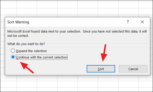
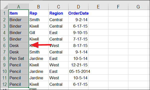
The selected column will be sorted independently, but be aware that this may lead to data misalignment across your worksheet.

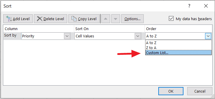
Sorting data in a custom order

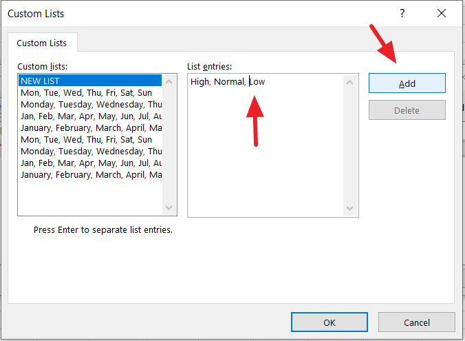
Sometimes, you might need to sort data based on a custom list, such as priorities or rankings that are specific to your dataset.

Click on any cell within your data and open the ‘Sort’ dialog box from the Data tab.

In the ‘Sort by’ dropdown, select the column you want to sort. Choose ‘Cell Values’ in the ‘Sort On’ dropdown, and select ‘Custom List’ from the ‘Order’ dropdown.

In the Custom Lists dialog box, enter your custom sort order in the ‘List entries’ box. For example, type ‘High’, ‘Normal’, ‘Low’, each on a new line, and click ‘Add’ to create the list.

Select your custom list and click ‘OK’ to return to the Sort dialog box. Your custom sort order will now appear in the ‘Order’ dropdown.

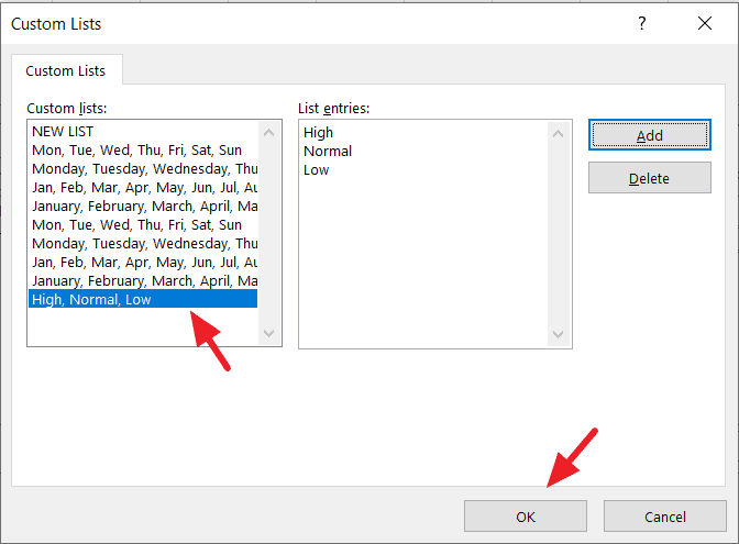
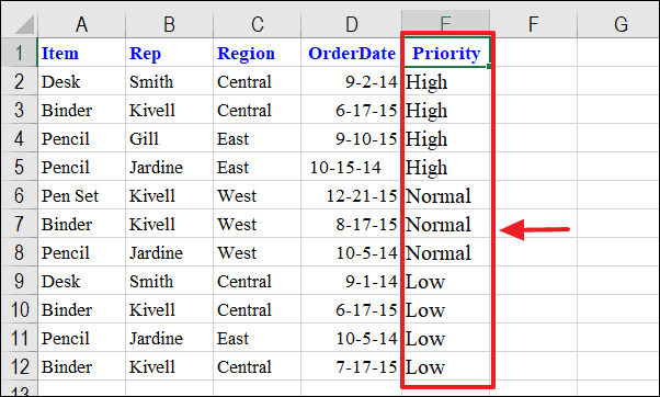
Click ‘OK’ to sort your data. The dataset will now be arranged according to your custom priority order.

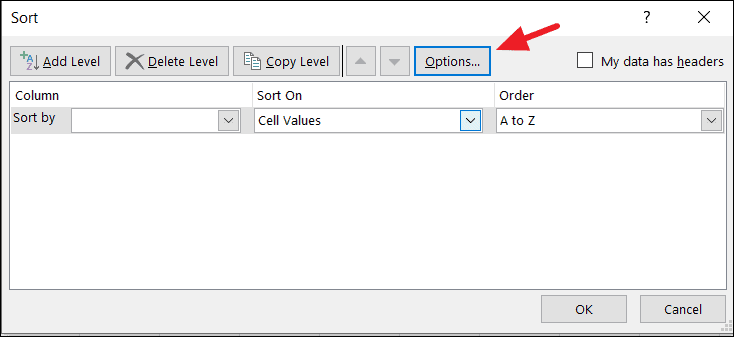
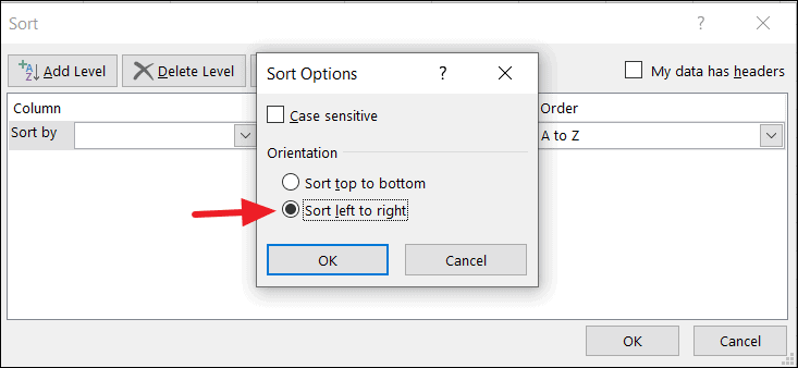
Sorting data in a row

Excel also allows you to sort data horizontally across rows instead of vertically down columns.

Select any cell in the row you wish to sort and open the ‘Sort’ dialog box from the Data tab.

In the Sort dialog box, click on the ‘Options’ button to access additional settings.

In the Sort Options dialog, select ‘Sort left to right’ under Orientation, and click ‘OK’.

Back in the Sort dialog box, choose the row you want to sort from the ‘Sort by’ dropdown, and set your sorting preferences.

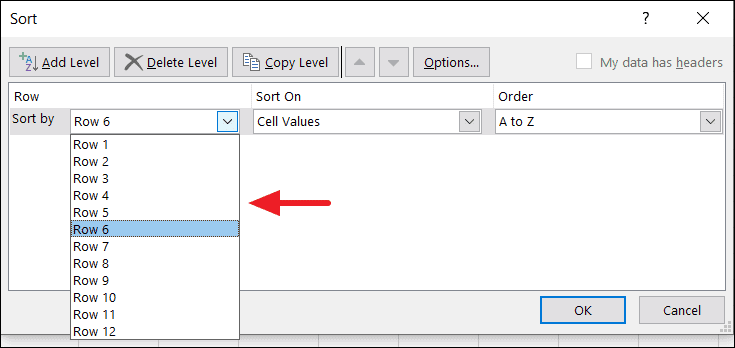
After clicking ‘OK’, your data will be sorted horizontally based on the values in the selected row.

By mastering these sorting techniques in Excel, you can efficiently reorganize your data to enhance readability and streamline your workflow.