In Excel, there are occasions when reorganizing data by swapping rows and columns can make your analysis more efficient or enhance the presentation of your information. Transposing data allows you to rotate your data table so that columns become rows and rows become columns.
How to Transpose Data in Excel Using Paste Special
The simplest method to transpose data in Excel is by using the Paste Special feature. This technique quickly converts your data orientation and preserves the original formatting, including any empty cells. However, keep in mind that the transposed data is static; changes made to the original data will not reflect in the transposed version.
Step 1: Select the range of cells that you want to transpose. For example, choose the entire table or data range that you wish to rotate.
Copy the selected cells by right-clicking and choosing Copy, or by pressing CTRL + C.
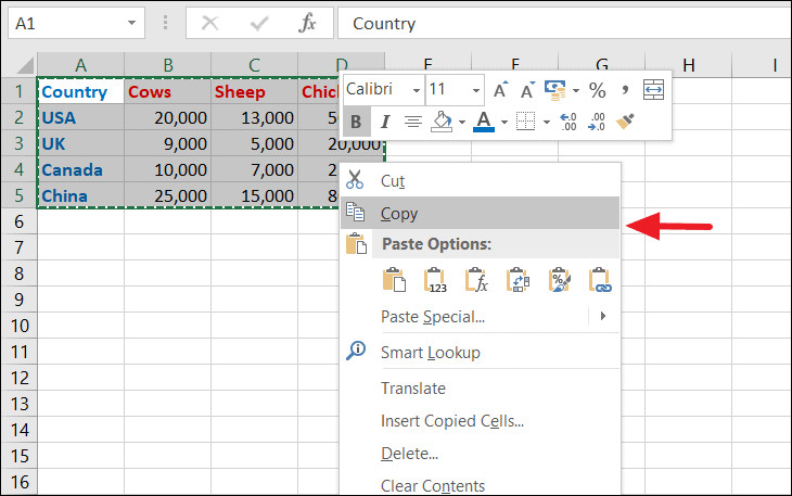
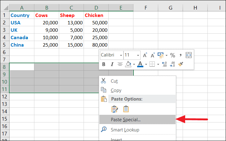
Step 2: Click on the cell where you want the transposed data to begin. Ensure that the area you select has enough space to accommodate the transposed data, with the number of rows and columns reversed.

Step 3: Right-click on the destination cell and select Paste Special from the context menu.
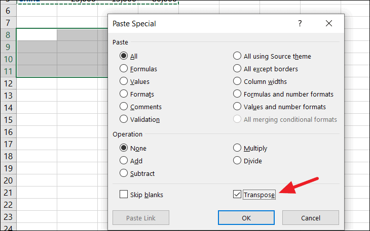
Step 4: In the Paste Special dialog box, check the Transpose option at the bottom. Then, click OK to paste the transposed data.
Step 5: The data will now appear in the new location with the rows and columns swapped. The original formatting, including any colors, fonts, and cell borders, will be preserved.
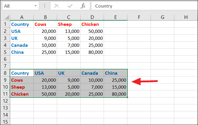
This method ensures that empty cells are accurately transposed without replacing them with zeros. It's an efficient way to reorganize data when you do not require the transposed data to update dynamically with changes in the original dataset.
How to Transpose Data Using the TRANSPOSE Function
The TRANSPOSE function in Excel offers a dynamic solution to transpose data. When you use this function, any updates made to the original data range will automatically reflect in the transposed data. However, the formatting from the original data is not retained, and you need to enter the formula as an array formula.
Step 1: Identify the data range you wish to transpose. For instance, suppose your data is in the range A1:D5, which comprises 5 rows and 4 columns.
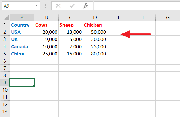
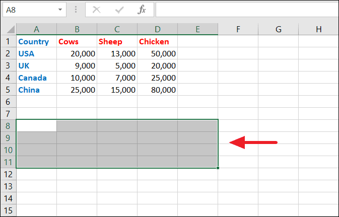
Step 2: Select a blank area in your worksheet where you want the transposed data to appear. The selected range should have the opposite dimensions of the original data range—in this example, 4 rows and 5 columns.
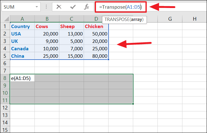
Step 3: With the destination range selected, type the TRANSPOSE function formula: =TRANSPOSE(A1:D5). Do not press Enter yet.
Step 4: Press Ctrl + Shift + Enter to enter the formula as an array formula. The transposed data will populate in the selected range.
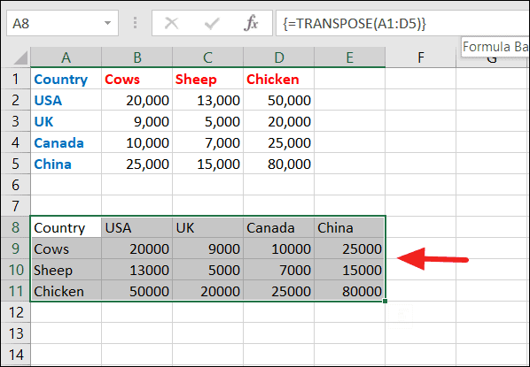
Using the TRANSPOSE function ensures that your transposed data stays up-to-date with the original data. However, note that this method does not carry over any formatting from the source data.
Transposing Data Without Zeros
When using the TRANSPOSE function, any empty cells in the original data may appear as zeros in the transposed data. To maintain empty cells without displaying zeros, you can use the IF function within your TRANSPOSE formula to check for blank cells.
Step 1: Modify your TRANSPOSE formula to include the IF function: =TRANSPOSE(IF(A1:D5="","",A1:D5)). This formula checks each cell in the range A1:D5; if a cell is empty, it returns an empty string (""); otherwise, it transposes the cell's value.
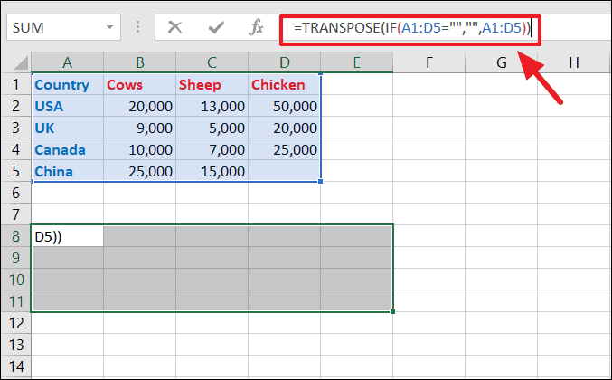
Step 2: Press Ctrl + Shift + Enter to apply the formula as an array formula. The transposed data will now accurately reflect empty cells without replacing them with zeros.
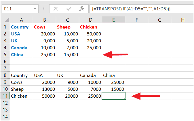
By incorporating the IF function, you ensure that your transposed data mirrors the original data more precisely, including the presence of empty cells.
Transposing data in Excel enhances the flexibility of your data presentation, allowing you to reorganize information to suit your needs. Whether you choose the straightforward Paste Special method or the dynamic TRANSPOSE function, Excel provides effective tools to rearrange your data efficiently.

