
The Search function is a text function that searches for a specific character or sub-string within another string or text and returns its position. In other words, it locates a word within another word and its position in the cell as an integer.
For instance, if you use the SEARCH function to find the position of the letter ‘s’ or the text ‘son’ in the word “Jackson”, it will return 5. It will only return the starting position of the search string in the searched cell.
The SEARCH function is rarely used alone, it is often used along with FIND, MID, LEFT, ISNUMBER, and others. In this article, we will explain what the SEARCH function is, how to use it, and how to use the SEARCH function combined with other functions in Excel.
Excel SEARCH Function
The SEARCH function looks for a text string or character within another text string and returns the starting position of the search string in the specified cell or the given string.
Syntax of the SEARCH function in Excel
=SEARCH (find_text, within_text, [start_num])find_text(required) is the character or string/text that you are searching for.within_text(required) is where you are searching the find_text. It is usually the cell reference that contains the text string we need to search. However, you can also input the string directly into the formula.[start_num](optional) specifies the position in the within_text string from where you want the search to begin. If omitted, the search will start from the first character of the within_text string.
The SEARCH function is not case-sensitive. If you are looking for a case-sensitive match, you can use the FIND function. If the function finds multiple matches for the search word, it will only return the position of the first word.
Search Function also supports the following wildcard operators:
- Question mark (?) is used to match any single character or letter with the text string.
- Asterisk (*) is used to match any number of characters with the string.
- Tilde (~) is used to match an actual question mark or asterisk. Type a tilde (~) before the other two wildcards to find them.
Search for a Character or Text in a Text String from the Beginning
You can use the SEARCH function to look for a specific character or text/word within a text string from the beginning and return its position. It searches the string from the first character, left to right, to the end of the string in the cell.
To search for a specific character or word in a text string, try the following formula:
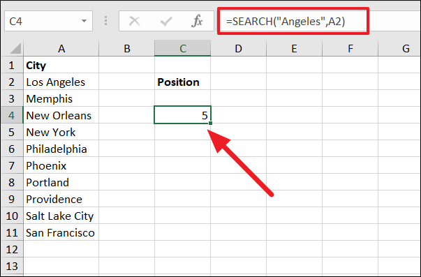
=SEARCH("Angeles",A2)or
To search from the beginning of the text string, you can either omit the last argument (start_num) or set it as 1:
=SEARCH("Angeles",A2,1)The above formula searches for the text ‘Angeles’ starting from the first character in the string ‘Los Angeles’ (A2) and returns the position of the starting point of the searched text (Angeles) – 5.
You can also use cell reference for the find_text argument in the formula:
=SEARCH(D3,A11,1)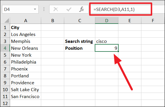
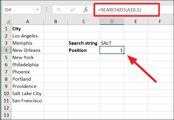
Case-Insensitive Search
As we mentioned earlier, the SEARCH function is not case sensitive, you can search for the word ‘SaLt’, ‘SALT’, or ‘Salt’ using the formula and it will return the same result no matter what case the find_text or within_text arguments uses.
Search for a Character(s) or Text in a Text String from Specific Starting Position
The SEARCH function can also be used to find the position of a word or text in a string by beginning the search at a specific point of within_text instead of the first character. By specifying the start number (start_num) in the formula, you can tell the function from where you want to start the search.
Example 1:
To search for a word from a specific position, try the below formula:
=SEARCH(C2,A2,9)Here, we specified the last argument (start_num) as 9. So the SEARCH function starts looking for the word Sparta (C2) from position 9 (from the space character after the word Ghost) in the string of cell A2 and returns the position of the search word as 14.
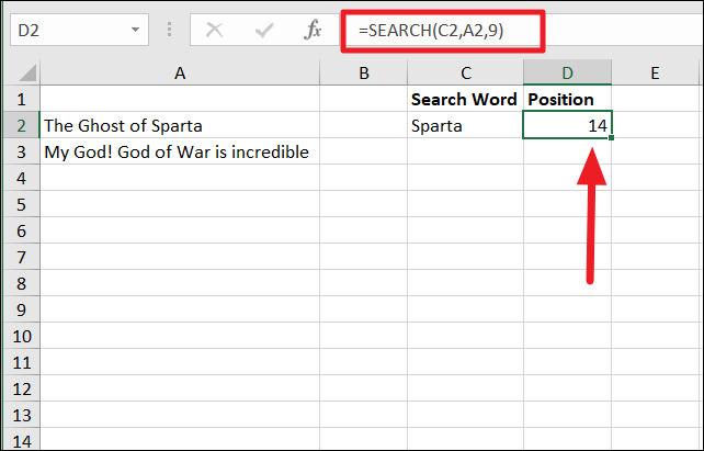
Remember, when counting positions, the space character is also included in the count.
When there are Multiple Occurrence of the Searched Text
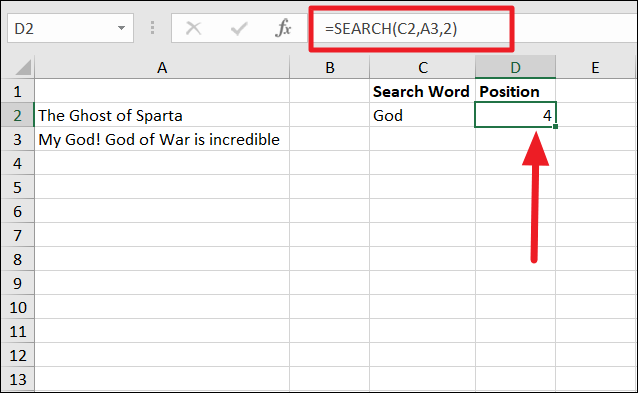
Let’s try another example. If we want to find the position of the word ‘God’, we can try the below formula:
=SEARCH(C2,A3,2)The start number (start_num) is 2 here, so the searching begins at the ‘y’ character. Although there are two instances of the word ‘God’ in the string, it only returns the position of the first word from the start number. Hence, the output is 4.
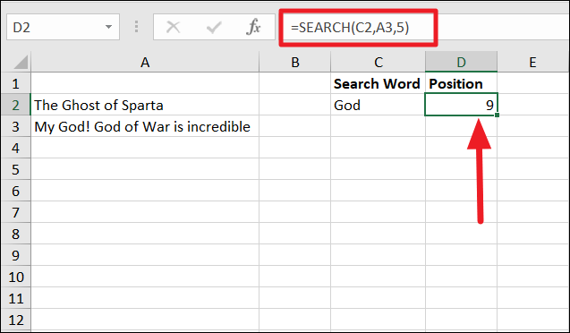
Now, let’s try changing the start number to 5:
=SEARCH(C2,A3,5)Now, you will get the output as 9, because the search begins at the character ‘o’ (in the first instance of the word God), and the first instance of ‘God’ is ignored.
#VALUE! error
There are two cases where you will get the ‘#VALUE!’ error when searching for the text with the SEARCH function:
- If the given search word (find_text) is not found in the specified within_text string.
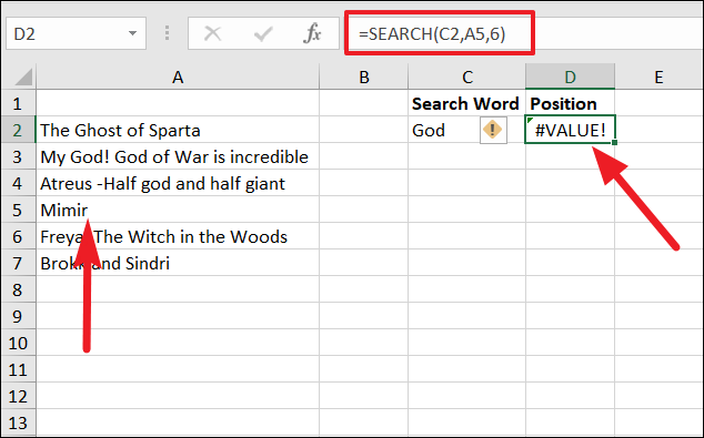
- If the starting number (start_num) is less than zero or greater than the length of the within_text string.
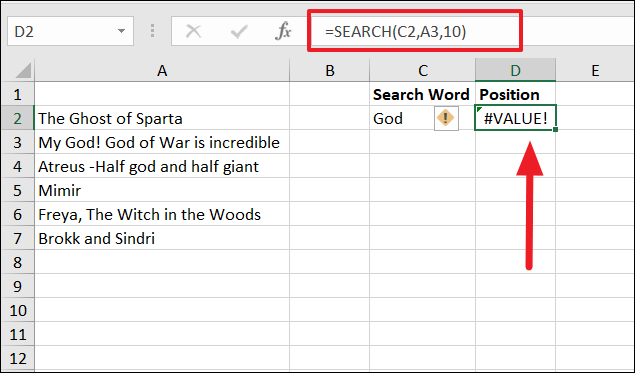
As you can see below, starting number for the search is 10. Both instance of the full word ‘God’ comes before position 10, hence the #VALUE! error.
In the below example, the starting number exceeds the length of the within_text string, so we get the #VALUE! error.
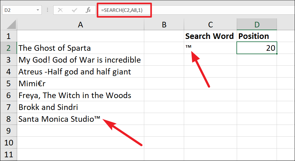
The SEARCH function can be used to find any kind of characters even symbols. For example, we searched for the location of the Trademark (™) symbol in the given string and found its position as 20.
Search with Wildcard Characters in Excel SEARCH function
SEARCH function supports wildcards – the question mark (?), an asterisk (*), and tilde (~). The question mark (?) represents any single character, the asterisk (*) denotes any series of characters, and the tilde (~) matches any of the other two wildcards.
Example 1:
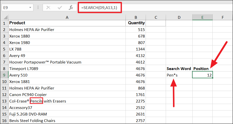
In the below example, wildcard (*) is used to find the position of the word ‘Pencils’ (Pen*S) in the string in cell A13:
=SEARCH(D9,A13,1)Here the search word is ‘Pen*s’ (D9), so the formula looks for any text that starts with ‘Pen’ and ends with ‘s’ and has any numbers of characters in between them in cell A13. It matches the text ‘Pencils’ and returns its position as 12.
Example 2:
When specifying starting number (start_num), you need to specify the correct start number to begin the search.
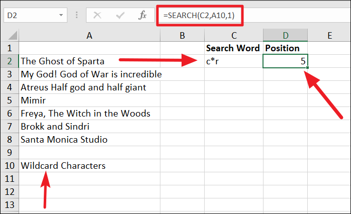
For example, the below formula can find the position of the text ‘c*r’ in the string of the cell A10:
=SEARCH(C2,A10,1)We wanted to find the position of ‘char’ in the word ‘character’ instead we got the position of ‘car’ in ‘Wildcard’, which is 5.
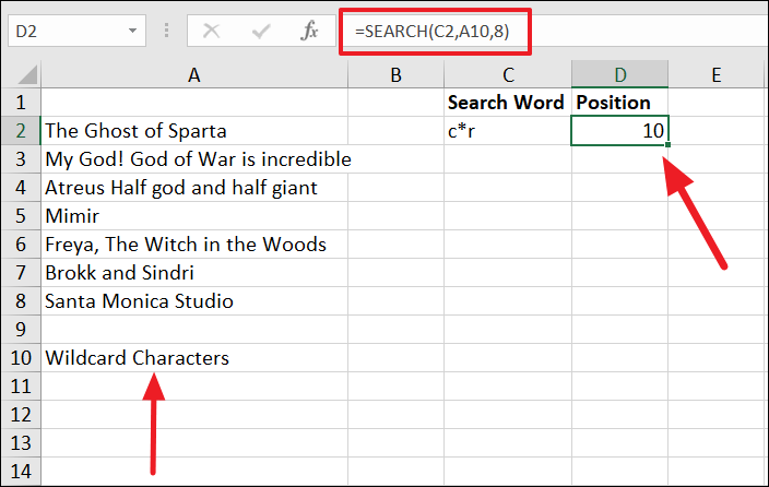
To fix this, we can change the starting number for searching to 8. Now the function starts the search from the character ‘d’ at the end of the wildcard and finds the position of ‘Char’ in ‘Characters’.
Example 3:
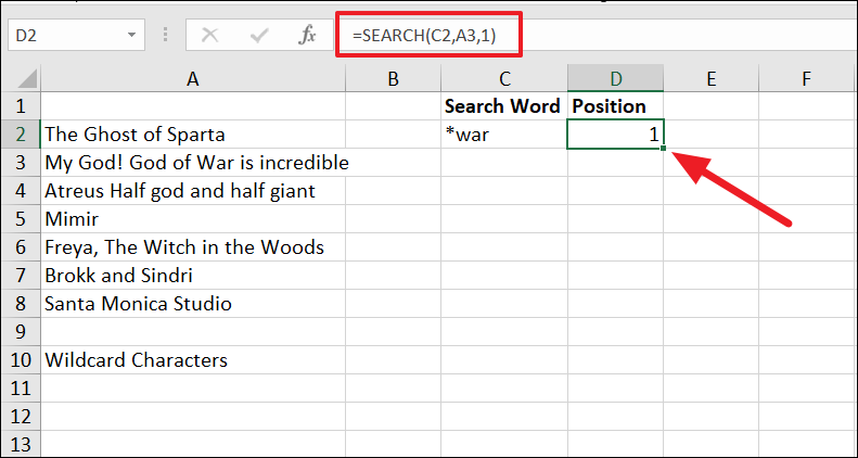
Another example where the wildcard used before the search word. Now no matter how many other characters there are in front of the ‘war’ in cell A3, it will return the position for the search as 1.
Example 4:
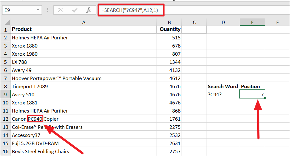
In the below example, question (?) is used to find the position of the text ‘PC940’ (?C94?) in the string in cell A12:
=SEARCH("?C94?",A12,1)Where ? denotes any single character, so the formula matches the string ‘PC940’ which is located at position 7.
Using SEARCH Function with Others Functions
The SEARCH function is usually combined with other functions such as MID, LEFT, RIGHT, or ISNUMBER to perform powerful calculations.
Find and Extract String using SEARCH Function
You can use the SEARCH function with LEFT, RIGHT, or MID functions to locate and extract a substring in a text string to the left or the right of a specific character, or between two characters. For instance, these combinations are helpful for splitting a list of full names into first names, last names, and middle names.
Extract a Substring Before Specific Character(s) using SEARCH and LEFT functions
If you have a text string or list of strings, you can use the SEARCH function in conjunction with the LEFT function to extract a substring or part of the string to a separate column.
The LEFT function helps you extract a specific number of characters from the left side of the string, starting with the first character of the string.
Syntax of LEFT function:
=LEFT(text,[num_chars])It requires two arguments:
textis the text string or reference to a cell that contains the characters you want to extract.num_charsis the number of characters you wish to extract from left to right in the giventext(this includes space between the characters).
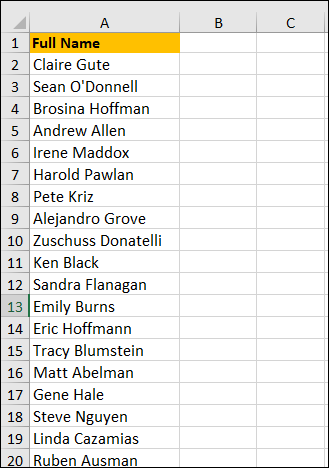
Suppose you have a list of full names in a column and you want to extract the First names into separate columns, you can do that with LEN and SEARCH functions. Here’s how it works:
The syntax for extracting a substring before a specific character:
Use the below formula (a combination of LEN and FIND) to extract a substring before a specific character:
=LEFT(text,SEARCH("char",text)-1)textspecifies the text string from which we want to extract a substring/text. It could be a text string or a reference to a cell that has the string.charis the specific character for which we want to determine the position.
The SEARCH function finds the position of the specified character in the given text string, then 1 is subtracted from that position number (position of the specified character) to determine the length of the substring to extract. Then the length is supplied to the LEFT to extract the number of characters from left to right in the string.
Example:
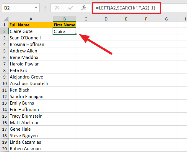
Enter the following formula to extract the first name from the full name:
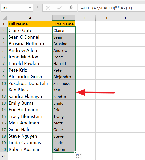
=LEFT(A2,SEARCH(" ",A2)-1)The above formula uses the SEARCH function to determine the position (which is 7) of the space character (“ “) in between the first and last name and subtracts 1 to exclude the space itself. Now we got the length of the first name (leftmost 6 characters). This number is then supplied to the LEFT function to return the number of characters (6) from left to right in the string.
If your list of strings has a pattern like they all have space characters in between. Then you can use Excel LEFT and FIND formula to extract strings from an entire column using auto-fill without having to specify the char argument for each formula.
To do that, select the formula cell (B2) and drag the fill handle (little green square at the bottom of the selected cell) down to other cells to apply this formula to a column. Now all first names have been extracted into column B as shown below:
Extract a Substring After Specific Character(s) using SEARCH and RIGHT
If you want to extract a substring after a specific character, you need to use the combination of the RIGHT, SEARCH, and LEN functions. The SEARCH and LEN function is nested in the num_char argument of the RIGHT function to find the number of characters to extract and the RIGHT function extract those characters.
The syntax for extracting a substring after a specific character:
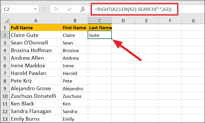
=RIGHT(text,LEN(text)-SEARCH("char",text))Suppose we have a column of full names and you want to extract the Last names into separate columns, you can do that with the following formula:
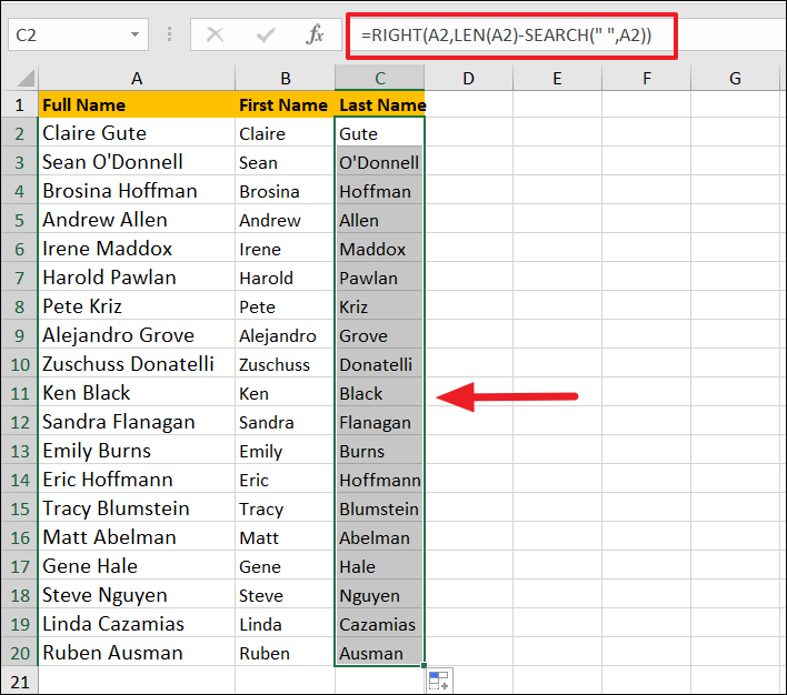
=RIGHT(A2,LEN(A2)-SEARCH(" ",A2))In the above formula, the SEARCH function returns the position of the space character ‘ ’, which is 7, and the LEN function finds the total number of characters in the string (string length). Then the position of the space is subtracted from the total number of characters in the string to find the length of the last name, which is supplied to the RIGHT function to extract that many characters from the end of the string.
Once the last name is extracted to a separate column, drag the fill handle down to other cells to apply this formula to the column. Now all the last names have been extracted into column C as shown below:
Extract a Substring Between Two Characters using MID and SEARCH Function
If you wish to extract the middle portion of the text string, you can do that with the help of MID and SEARCH functions.
Excel MID Function
The MID Excel Function is used to extract a middle portion of a string. To do that, it requires the text string, a starting point (position), and the number of characters to extract.
Syntax:
=MID(text,start_num,num_chars)textspecifies the text string from which we want to extract a substring/text. It could be a text string or a reference to a cell that has the string.start_numspecifies the position in the text string from where you want the start the extraction. If omitted, the search will start from the first character of the within_text string.num_charsis the number of characters you wish to extract from left to right in the giventext.
The start_num and num_chars arguments can be supplied by the SEARCH function to the MID function to extract a substring between two characters.
Let us see how the MID function works with this simple example:
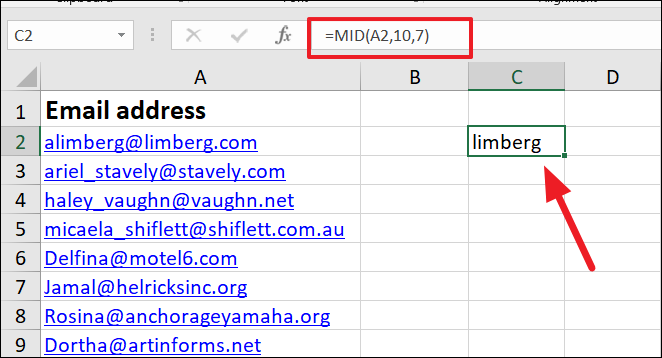
=MID(A2,10,4)The formula counts the characters in cell A2 from left to right until it gets to the 10th character and then it returns the next 7 characters (including the 10th character).
To extract a substring between two characters with MID and SEARCH, use the following syntax:
=MID(text,SEARCH("char",text)+1,SEARCH("char",text)-SEARCH("char",text)-1)text: A string from which we wish to extract a substring, this could be a text string or a reference to a cell that has a string.char: A specific character for which we want to determine the position.
Example 1:
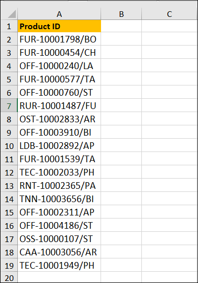
Suppose you the column of Product IDs and you want to extract ID numbers between ‘-‘ and ‘/’ characters.
We need to find positions of the two specified characters, then subtract the position of the 2nd given character from the position of the 1st character, and subtract 1 from the result to determine how many characters to extract starting from the position of the first character.
To extract the middle string between two characters, enter this formula into a blank cell:
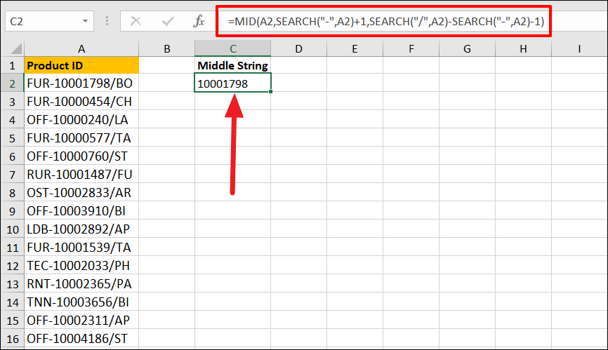
=MID(A2,SEARCH("-",A2)+1,SEARCH("/",A2)-SEARCH("-",A2)-1)Explanation:
A2is the cell that contains the original text string from which we want to extract the substring.SEARCH("-",A2)+1(start_num) determines the position of the first specified character (-) and adds 1 to start the extraction from the next character (start_num=5).SEARCH("/",A2)-SEARCH("-",A2)-1(num_chars) finds the length of the substring we want to extract between ‘-‘ and ‘/’ characters by subtracting the position of ‘/’ (13) from the position of ‘-’ (4) and subtracting 1 from the result. This will tell the MID function how many characters to extract.
Now, the MID function knows how many characters to extract from the string and where to start. It will return the middle string in cell C2.
After that, you can copy the formula to the rest of the cells to extract the middle string for the whole column.
Example 2:
The MID and SEARCH are really useful when extracting middle names from a list of full names. To extract the middle name, use this formula:
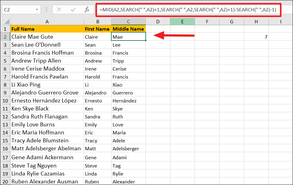
=MID(A2,SEARCH(" ",A2)+1,SEARCH(" ",A2,SEARCH(" ",A2)+1)-SEARCH(" ",A2)-1)The problem is both specified characters are space characters (same), so the formula won’t be able to distinguish between which is which, and it will result in #VALUE!. To fix this, we nested a SEARCH function inside another SEARCH function and added 1 in the ‘num_chars’ argument to find the position of the second space character.
SEARCH(" ",A2)+1determines the starting point for extraction by adding 1 to the position of the first space character.SEARCH(" ",A2,SEARCH(" ",A2)+1)-SEARCH(" ",A2)-1subtracts the position of the 2nd space from the position of the 1st space and subtracts 1 from the result to remove a trailing space. The resulting value tells the formula how many characters to extract.
Now with the original text string, starting number, and the number of characters, the MID function extracts the middle name from the full name (A2).
Find Nth Occurrence or Position of a Character in a String using SEARCH function
If you are trying to find the position of a character or text that occurs multiple times in a string, the SEARCH function will only return the first match of that character/text. However, when you combine the SEARCH and SUBSTITUTE functions, you can find the nth occurrence or position (such as the second or third instance) of a specific character (or string of characters) in a text string easily.
Here’s the generic formula for finding the position of the Nth occurrence of a character:
=SEARCH(CHAR,SUBSTITUTE(text, character, CHAR, [instance_num])) where
CHARis a function that returns a symbol based on its ASCII code. You can use any ASCII code or the symbol that you are sure will not appear in the string.textis the text string or reference to a cell that contains the string from which you want to find the nth occurrence.characteris the character for which you want to find the nth occurrence.[instance_num]specifies which occurrence of the character(s) or text string you would like to find.
Example 1:
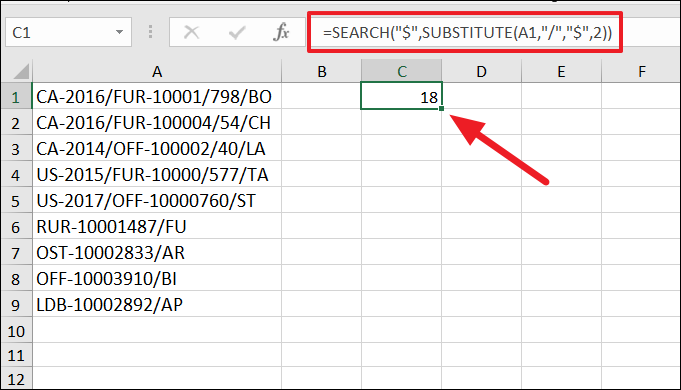
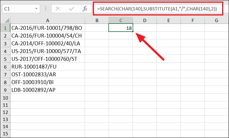
In the below example we want to find the 2nd occurrence of the character ‘/’ with the following formula:
=SEARCH("$",SUBSTITUTE(A1,"/","$",2))The SUBSTITUTE function actually searches for a character or text and replaces it with another. In the above formula, we’re substituting the character (/) with ‘$’, which won’t show up in the string. So when the SUBSTITUTE function replaces the 2nd occurrence of the character ‘/’ in the string for the symbol ‘$’, the SEARCH returns the position of that character.
You can also use CHAR ASCII code in the CHAR argument of the formula for substituting search characters (/) to get the same results.
Example 2:
Another formula that can help you find the nth occurrence of a specific character from the text string.
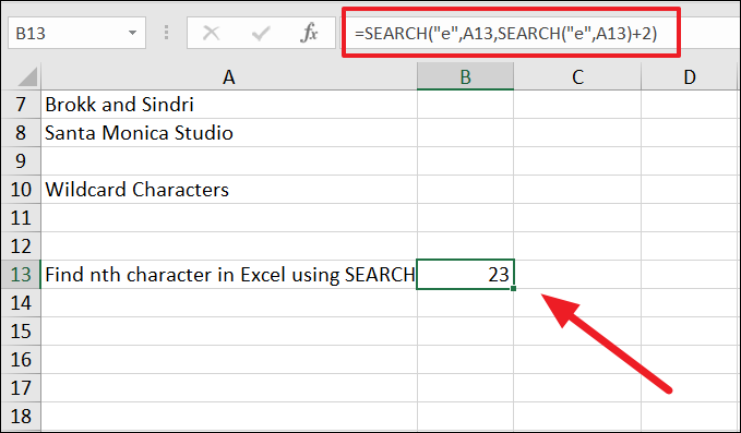
The below formula will return the position of the 3rd occurrence of “e” in cell A1:
=SEARCH("e",A13,SEARCH("e",A13)+2)The above formula will return the position of 3rd ‘e’ as 23. You can specify the occurrence in the formula by changing the last argument (2) accordingly. If you want to find the first occurrence of “e”, change 2 to 0. And to find the second occurrence of “e”, change 2 to 1, and so on.
Combine ISNUMBER with SEARCH function to Check Specific Text
As we know, the SEARCH function searches for a specific substring within a string and returns its numerical position if the text is found otherwise it returns a #VALUE! error. The ISNUMBER function checks if a cell contains a number or not. If yes, it returns TRUE, otherwise, it returns FALSE.
However, when the ISNUMBER function combined with the SEARCH function, it can check if a cell contains specific text and return TRUE if the text is found, otherwise it returns FALSE.
Here’s the generic formula to check if a cell contains the specific text:
=ISNUMBER(SEARCH(substring,text))Where
substringis the text string that you wish to findtextis the cell or string where you want to check for the substring.
Example:
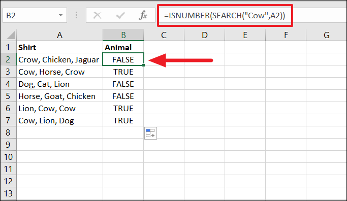
In the below dataset, we want to find whether the word Cow exists in column A:
=ISNUMBER(SEARCH("Cow",A2))First, enter the formula in cell A2, and auto-fill the formula to the column. The ISNUMBER function checks whether the string ‘Cow’ appears in cell A2 and returns FALSE.
The SEARCH function checks cell A2 for the text ‘Cow’ and returns the ‘#VALUE!’ error (because the text Cow is not present). The ‘#VALUE!’ is not a number so the ISNUMBER function returns ‘FALSE’. In cell B2, the SEARCH function checks for the word ‘Cow’ and return its position number, so the ISNUMBER returns ‘TRUE’.
We can also use a cell reference to input string into the formula:
=ISNUMBER(SEARCH(B$1,A2))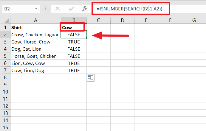
Check for Specific Text with IF, ISNUMBER, and SEARCH function
If you want to get something other than TRUE or FALSE when a substring is found in a string, you can use the IF function with ISNUMBER and SEARCH.
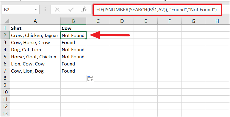
For example, we will try to find out whether each cell in column A contains the word ‘Cow’ and return “Found” if a cell contains that text, and “Not Found” if not:
=IF(ISNUMBER(SEARCH(B$1,A2)), "Found","Not Found")You can copy the formula in cell B2 to the rest of the cells using the fill handle. In the formula, the SEARCH function checks for the value in B1 against cell A1 and returns an error. So, the ISNUMBER function returns FALSE. As a result, the IF function returns ‘Not Found’.
That’s it.


