
Google has introduced a new, smart ‘formula suggestions feature’ in Google Sheet, which makes it easier to work with formulas and functions and helps make data analysis faster and easier. The new intelligent, content-aware suggestions feature will suggest you formulas and function based on the data you’ve entered on your spreadsheet.
This feature is added to Google Sheets by default but you can disable it anytime you want. To use this feature, all you have to do is start writing a formula, Sheets will show you a series of suggestions for functions and formulas based on the context of your data. Let us see how to use Formula Suggestions in Google Sheets with a few examples.
Using Intelligent Formula Suggestions in Google Sheets
Google Sheets can now auto-suggest formulas, much like the auto-complete feature available in Google Docs. When you start writing the formula by typing the ‘=” sign in the cell, formula suggestions will appear which can be incorporated into a spreadsheet with a press of the Tab key or by click on one of the suggestions.
The formula suggestions feature is trained with machine learning technology to make intelligent formula suggestions based on the data you’ve entered. Mind you, this feature does not work with every kind of data you’ve entered in your spreadsheets, it can only make suggestions if it understands the context and pattern of the data.
Example 1: SUM a Range of Cells using Intelligent Suggestions
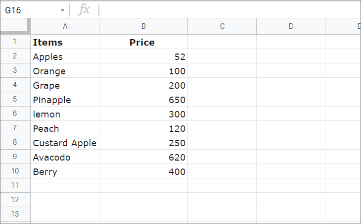
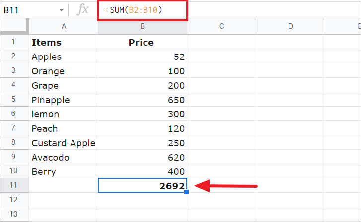
Let’s assume, you have the below data in your spreadsheet and you want to find the total price amount of all the fruits. For that, you would normally use the ‘SUM’ function to sum the values in the range B2:B10.
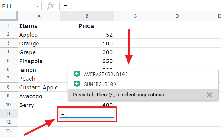
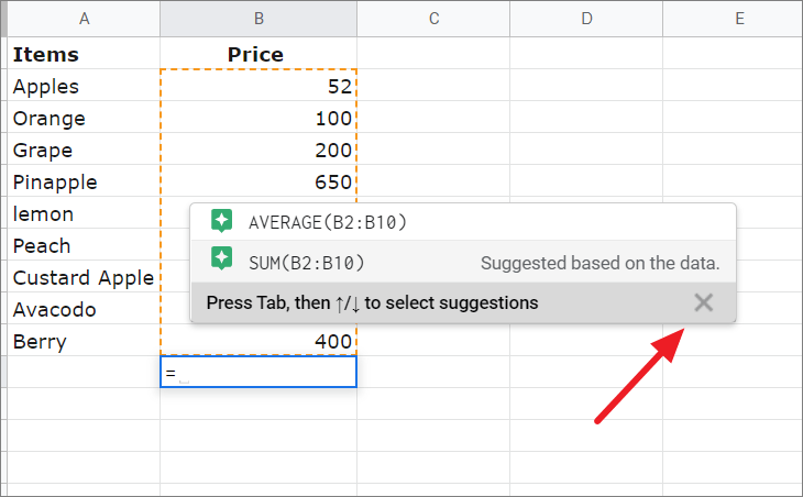
But with the smart suggestion feature, you don’t have to manually enter the whole formula. All you have to do is type ‘=’ sign in the cell (B11) below the range of data, and then the Google sheets will show you suggestions.
When you type ‘=’ in cell B11, Google Sheets will show you a list of suggested formulas and functions as shown below. As you can see, two data analysis formulas show up in the suggestions. Also, make sure to enter the ‘=’ sign in the cell at the bottom of the range or next to the reference/range you want to use to calculate.
Now, you want to calculate the total price, for that you would need the SUM formula.
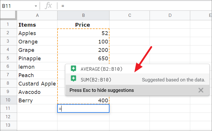
To select a suggested formula, press the Tab key on your keyboard or just click on one of the suggestions. Once, you pressed the Tab key, use the up and down arrow keys to select a suggestion, and then press Enter to insert the formula. Here, we’re selecting ‘=SUM(B2:B10)’.
If you don’t want the suggestions, press the Esc key or click the ‘X’ button on the suggestion box.
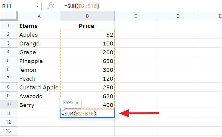
Once you selected the formula from the suggestions, it will be inserted in the cell but not executed. Now, you can make changes to your formula if you want, like changing parameters, range, etc. To execute the inserted formula, press Enter again.
This will output the result and move on to the next cell.
If you would like to work without these smart suggestions, you can disable them anytime you want. This feature can be disabled by clicking the ‘X’ icon on the suggestions box that appears or by pressing F10. Alternatively, you can turn off this feature by going to the ‘Tools’ menu and selecting ‘Enable formula suggestions’ from Preferences.
Example 2: Show Maximum Value from a Range of Cells with Intelligent Suggestions
In the previous example, since we entered a range of numbers (Sales amount), Google Sheets easily assumed that we probably wanted the total sum or average of the numbers and automatically suggested both formulas. But what if we want to calculate some other calculations? Is it smart enough to suggest formulas other than obvious ones? Let’s try this smart suggestion with another example.
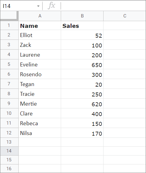
In the below example, we have a list of salespersons and their sales in two columns. Now, we want to find what is the highest sale on the list. Let’s see if we can do that with smart formula suggestions.
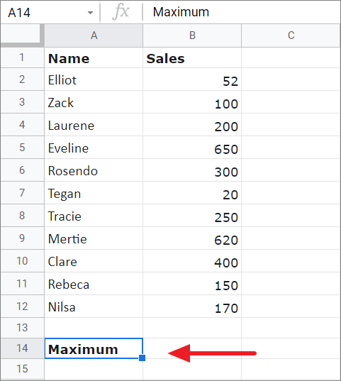
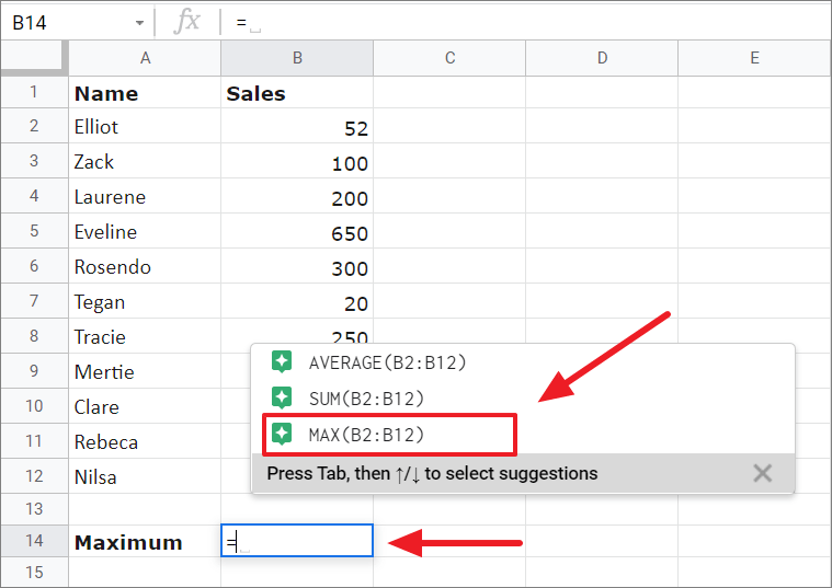
Let’s add a label named ‘Maximum’ at the bottom of the range in cell A14 and see if Google Sheets can recognize the label and suggest a formula according to that when we start writing.
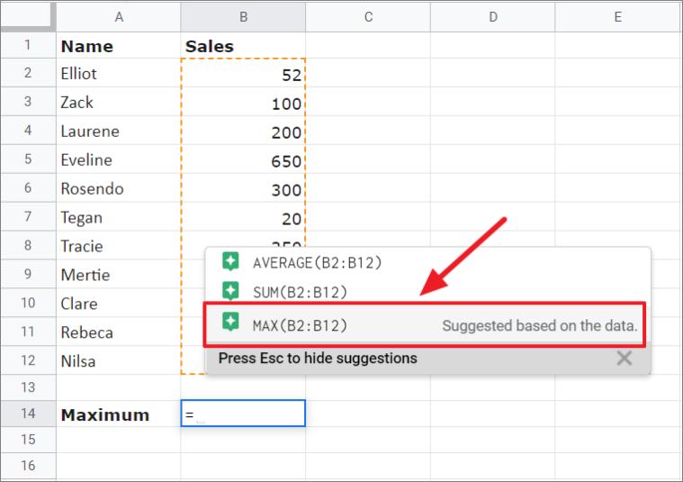
Now, when we enter the ‘=’ sign in the cell next to the label, at the bottom of the range, Sheets is smart enough to recogzise the label and the range of numbers and suggest us not only the ‘SUM’ and ‘AVERAGE’ formulas but also the ‘MAX’ function (which we want).
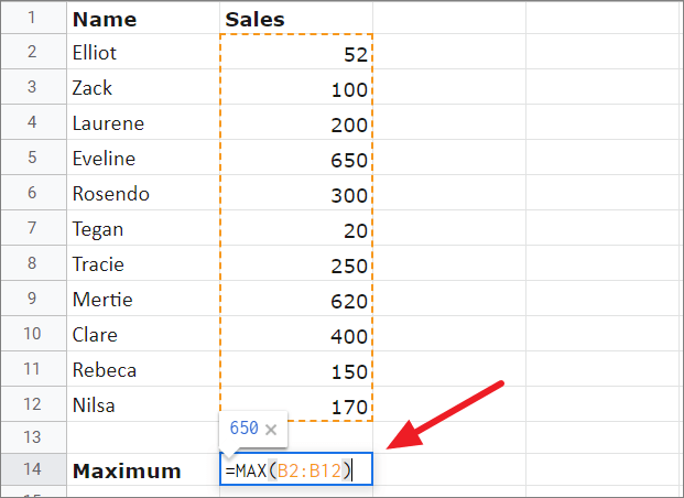
Then, press the TAB key to select the MAX() formula, and press Enter to accept the suggested formula.
Then, press Enter again to execute the formula.
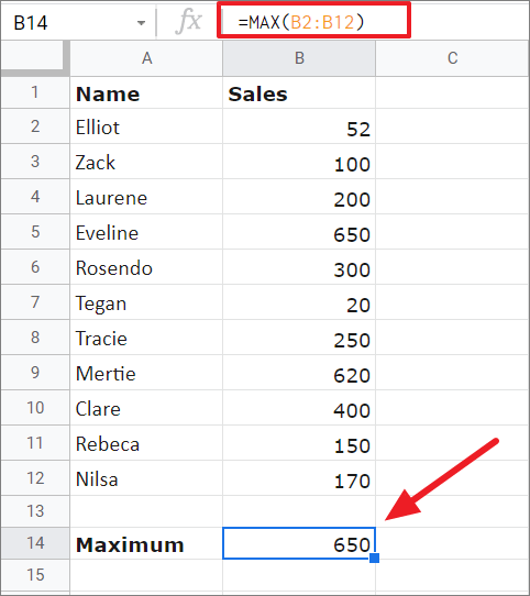
Now, we got the highest sales amount (maximum) from the list.
These formula suggestions can help you write formulas accurately and analyze data much quicker. It also helps us avoid formula errors which we often make by misspelling the syntax, entering wrong arguments, or missing comma or brackets. This feature is really helpful for new formula users in Google Sheets and it makes it easier for them to work with formulas and functions.
That’s it.