The ‘less than or equal to’ operator (<=) in Excel is an essential tool for comparing values and making logical decisions in formulas. This operator evaluates whether a value is less than or equal to another and returns ‘TRUE’ if the condition is met or ‘FALSE’ if not. It’s particularly powerful when combined with functions like IF, SUMIF, and COUNTIF to perform complex calculations.
Using ‘<=’ Operator with Functions
In Excel, logical operators like ‘<=’ are often used within functions to perform conditional calculations. By integrating these operators with functions, you can create dynamic formulas that respond to your data.
Using ‘<=’ with IF Function in Excel
The IF function works seamlessly with the ‘<=’ operator to perform logical tests and return specific values based on the outcome. For example, suppose you have a list of student scores and you want to determine if each student has passed or failed based on a passing score of 50.
Use the following formula in cell C2 to check the score in B2:
=IF(B2<=50,"Fail","Pass")This formula checks if the value in B2 is less than or equal to 50. If the condition is ‘TRUE’, it returns “Fail”; otherwise, it returns “Pass”.
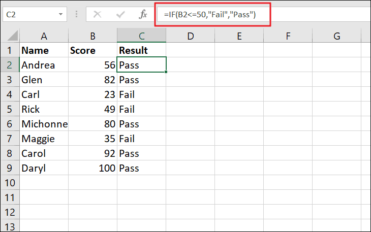
Copy this formula down the column to evaluate all the scores.
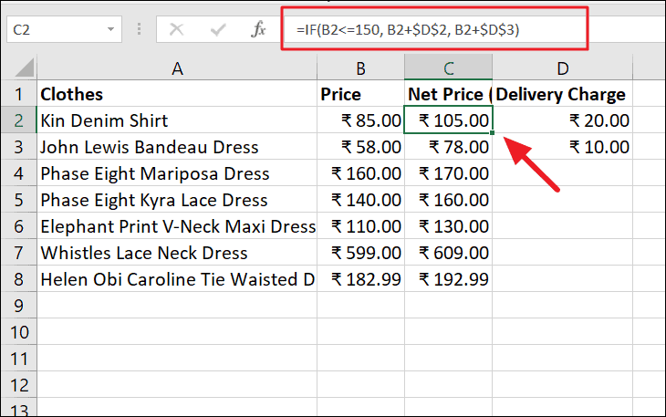
Another example involves calculating delivery charges based on the price of items. If an item’s price is less than or equal to $150, a delivery charge of $20 is added; otherwise, a charge of $10 is applied. Here’s the formula:
=IF(B2<=150, B2+$D$2, B2+$D$3)In this formula, ‘$D$2’ and ‘$D$3’ are absolute references to the cells containing the delivery charges. The formula adds the appropriate delivery charge to the item’s price in B2 based on the condition.
Using ‘<=’ with SUMIF Function in Excel
The SUMIF function sums values that meet a specific condition. By using the ‘<=’ operator in the criteria, you can sum all values less than or equal to a certain number or date.
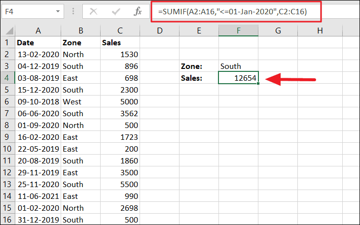
For instance, to sum all sales amounts on or before January 1, 2020, use the following formula:
=SUMIF(A2:A16,"<=1/1/2020",C2:C16)This formula checks dates in the range A2:A16 and sums the corresponding sales amounts in C2:C16 where the date condition is met.
Using ‘<=’ with COUNTIF Function in Excel
The COUNTIF function counts the number of cells that meet a certain condition. Using ‘<=’ allows you to count how many values are less than or equal to a specific number.
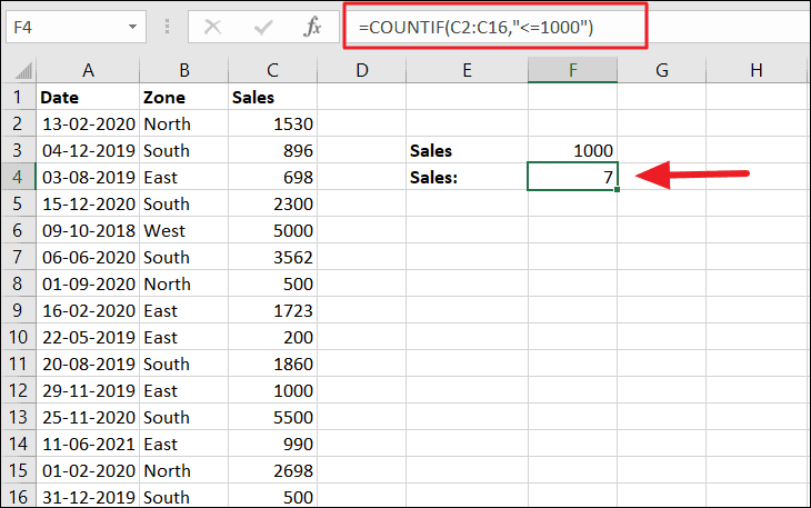
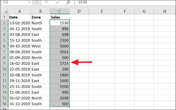
To count the number of sales less than or equal to 1000 in the range C2:C16, the formula is:
=COUNTIF(C2:C16,"<=1000")This formula returns the count of cells in C2:C16 where the sales amount is less than or equal to 1000.
If you have the criterion value in a cell, say F3, you can reference it in the formula:
=COUNTIF(C2:C16,"<="&F3)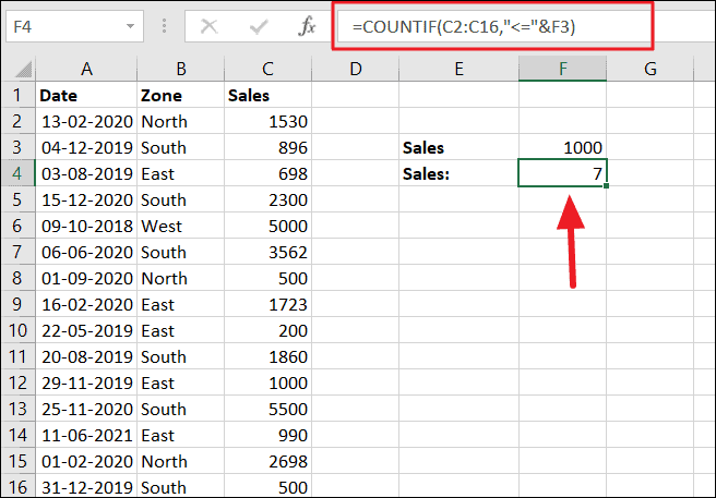
Compare Numbers with ‘<=’ Operator in Excel
Comparing numbers using the ‘<=’ operator is straightforward. It allows you to evaluate whether a numeric value is less than or equal to another number.
For example, to compare the values in cells A2 and B2, use the formula:
=A2<=B2This formula returns ‘TRUE’ if the value in A2 is less than or equal to the value in B2; otherwise, it returns ‘FALSE’.
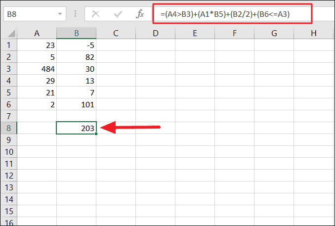
You can also incorporate the ‘<=’ operator into more complex mathematical calculations by combining it with other operators and functions. For example:
=(A4>B3)+(A1*B5)+(B2/2)+(B6<=A3)In this formula, logical expressions like ‘(A4>B3)’ and ‘(B6<=A3)’ evaluate to 1 for ‘TRUE’ and 0 for ‘FALSE’, contributing to the overall calculation.
Compare Dates with ‘<=’ Operator in Excel
The ‘<=’ operator can also compare dates in Excel. Since Excel stores dates as serial numbers, you can perform logical operations directly on date values.
For example, to check if the date in A2 is less than or equal to the date in B2, use:
=A2<=B2This formula compares the serial numbers of the dates, returning ‘TRUE’ if the condition is met.
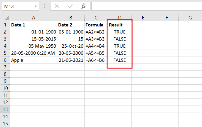
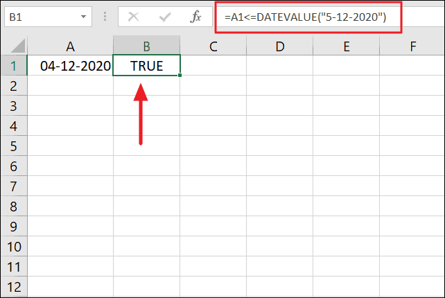
Be cautious when using dates directly in formulas, as Excel might interpret them incorrectly. To ensure accuracy, use the DATEVALUE function when comparing to a specific date:
=A1<=DATEVALUE("5-12-2020")This formula converts the date string into a serial number that Excel recognizes as a date.
Compare Text Values with ‘<=’ Operator in Excel
The ‘<=’ operator can be used to compare text strings in Excel. When comparing text, Excel evaluates the alphabetical order based on each character’s Unicode value. Note that logical operators are case-insensitive, so “A” and “a” are considered equal.
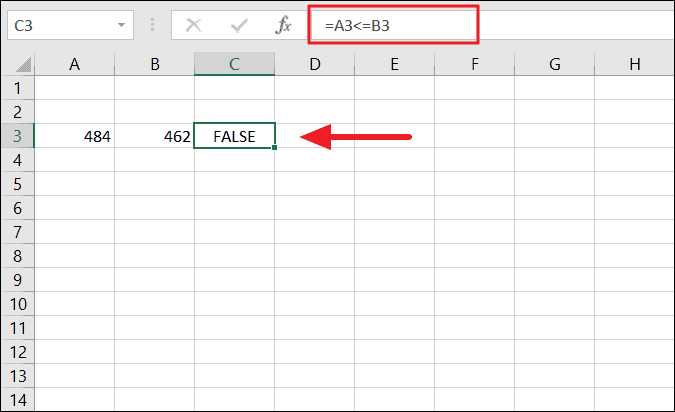
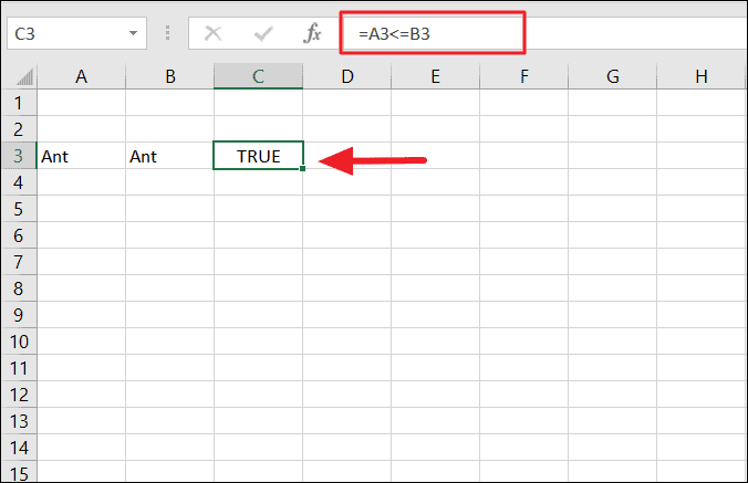
For example, to compare the text in cells A3 and B3:
=A3<=B3If both cells contain the same text, the formula returns ‘TRUE’.
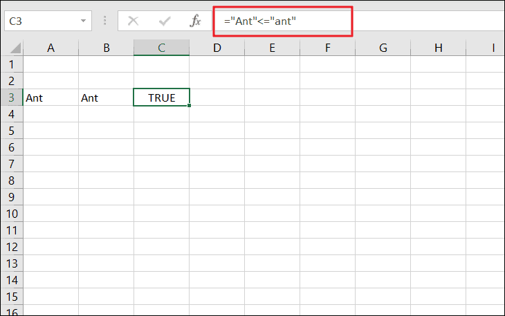
You can also compare text literals directly:
="Ant"<="ant"This formula returns ‘TRUE’ because Excel ignores case differences.
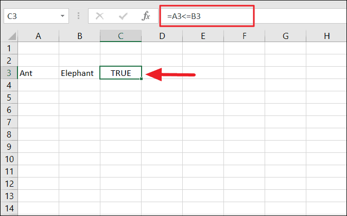
Example 1: Comparing “Ant” and “Elephant”:
Although “Ant” and “Elephant” are different, Excel compares them character by character. Since “A” is less than “E”, the formula:
=A3<=B3returns ‘TRUE’.
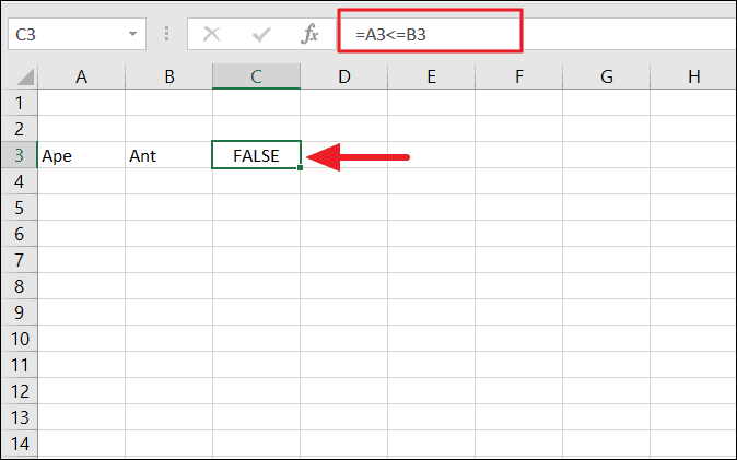
Example 2: Comparing “Apple” and “April”:
If the first letters are the same, Excel moves to the next character. In this case, “p” is not less than “p”, so it continues comparing. Eventually, it finds that “l” is less than “r”, and the formula:
=A3<=B3returns ‘FALSE’.
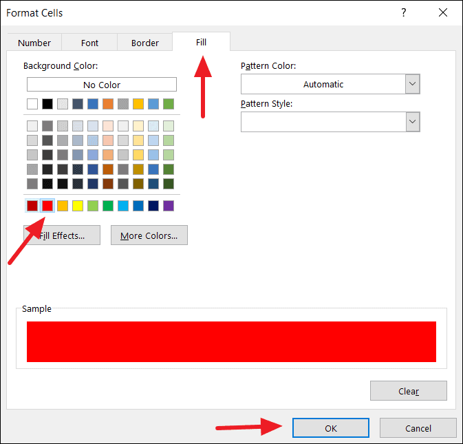
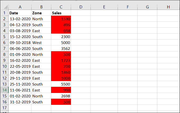
Using ‘<=’ Operator in Excel Conditional Formatting
The ‘<=’ operator is useful in conditional formatting to highlight cells that meet certain criteria. For example, to highlight sales amounts less than or equal to 2000, follow these steps:
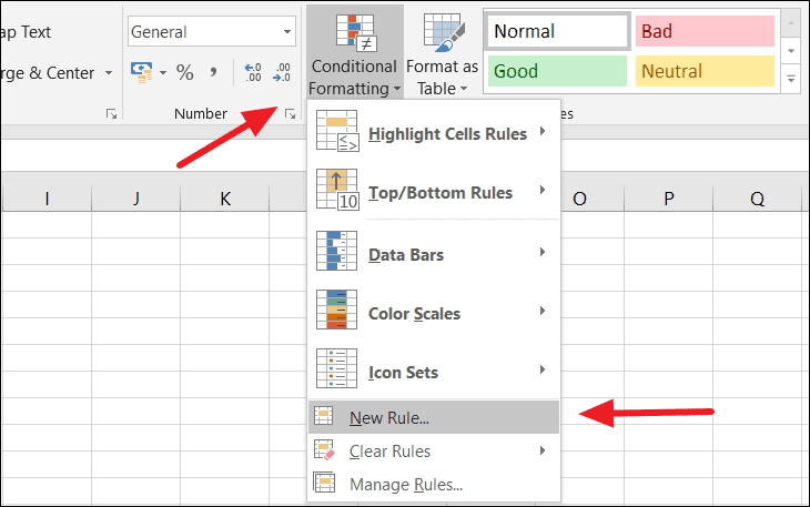
=C2<=2000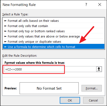
The ‘<=’ operator is a versatile tool in Excel that enhances your ability to perform logical comparisons and conditional calculations across various data types.


