
SUMIF is one of the mathematical functions in Google Sheets, which is used to conditionally sum cells. Basically, the SUMIF function looks for a specific condition in a range of cells and then adds up the values that meet the given condition.
For example, you have a list of expenses in Google sheets and you only want to sum up the expenses that are above a certain max value. Or you have a list of order items and their corresponding amounts, and you only want to know the total order amount of a specific item. That’s where the SUMIF function comes in handy.
The SUMIF can be used to sum values based on number condition, text condition, date condition, wildcards as well as based on empty and non-empty cells. Google Sheets has two functions to sums up values based on criteria: SUMIF and SUMIFS. SUMIF function adds up numbers based on one condition while SUMIFS sums numbers based on multiple conditions.
In this tutorial, we will explain how to use the SUMIF and SUMIFS functions in Google Sheets to sum numbers that meet a certain condition(s).
SUMIF Function in Google Sheets – Syntax and Arguments
The SUMIF function is just a combination of the SUM and IF function. The IF function scans through the range of cells for a given condition, and then the SUM function sums the numbers corresponding to the cells that meet the condition.
Syntax of SUMIF Function:
The syntax of SUMIF function in Google Sheets is as follows:
=SUMIF(range, criteria, [sum_range])Arguments:
range – The range of cells where we look for the cells that meet the criteria.
criteria – The criteria that determine which cells need to be added. You can base the criterion on the number, text string, date, cell reference, expression, logical operator, wildcard character as well as other functions.
sum_range – This argument is optional. It is the data range with values to sum if the corresponding range entry matches the condition. If you don’t include this argument, then the ‘range’ is summed instead.
Now, let us see how to use the SUMIF function to sum values with different criterion.
SUMIF Function with Number Criteria
You can sum numbers that meet certain criteria in a range of cells, by using one of the following comparison operators to make criteria.
- greater than (>)
- less than (<)
- greater than or equal to (>=)
- less than or equal to (<=)
- equal to (=)
- not equal to (<>)
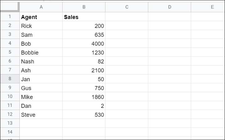
Suppose you have the following spreadsheet and you are interested in the total sales that are 1000 or higher.
Here’s how you can enter the SUMIF function:
First, select the cell where you want the output of the sum to appear (D3). To sum up numbers in B2:B12 that are greater than or equal to 1000, type this formula and press ‘Enter’:
=SUMIF(B2:B12,">=1000",B2:B12)In this example formula, the range and sum_range arguments (B2:B12) are the same, because sales numbers and criteria are applied on the same range. And we entered the number before the comparison operator and enclosed it in quotation marks because the criteria should always be enclosed in double quotation marks except for a cell reference.
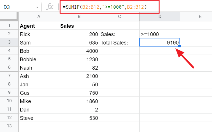
The formula looked for numbers that are greater than or equal to 1000 and then added up all the matched values and showed the result in cell D3.
Since the range and sum_range arguments are the same, you can achieve the same result without the sum_range arguments in the formula, like this:
=SUMIF(B2:B12,">=1000")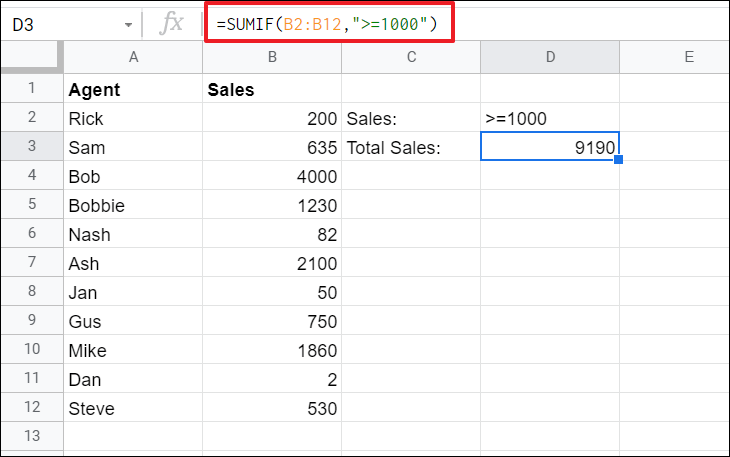
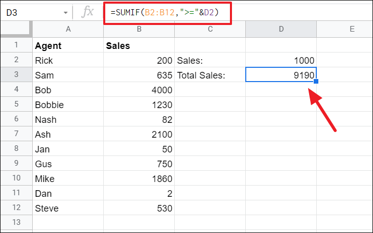
Or you can supply the cell reference (D2) that contains the number instead of the number criteria, and join the comparison operator with that cell reference in the criteria argument:
=SUMIF(B2:B12,">="&D2)As you can see the comparison operator is still entered in double quotation marks and the operator and cell reference are concatenated by an ampersand (&). And you don’t need to enclose cell reference in quotation marks.
Note: When you refer to the cell that contains criteria, make sure not to leave any leading or trailing space in the value in the cell. If your value has any unnecessary space before or after the value in the referred cell, then the formula will return ‘0’ as a result.
You can also use other logical operators the same way to make conditions in the criteria argument. For example, to sum values less than 500:
=SUMIF(B2:B12,"<500")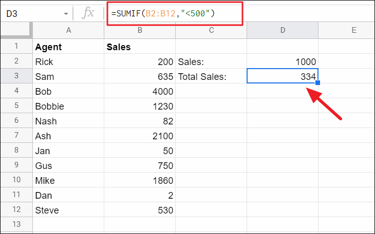
Sum If Numbers Equal to
If you want to add numbers that equal to a certain number, you can either enter only the number or enter the number with the equal sign in the criterion argument.
For instance, to sum the corresponding sales amounts (column B) for quantities (column C) whose values is equal to 20, try any of these formulas:
=SUMIF(C2:C12,"=20",B2:B12)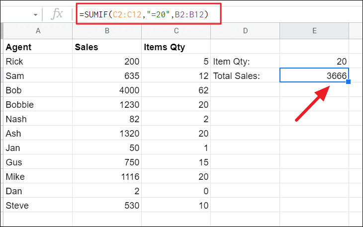
=SUMIF(C2:C12,"20",B2:B12)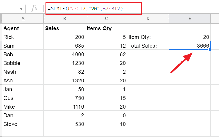
=SUMIF(C2:C12,E2,B2:B12)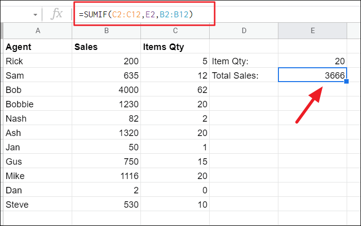
To sum numbers in column B with quantity not equal to 20 in column C, try this formula:
=SUMIF(C2:C12,"<>20",B2:B12)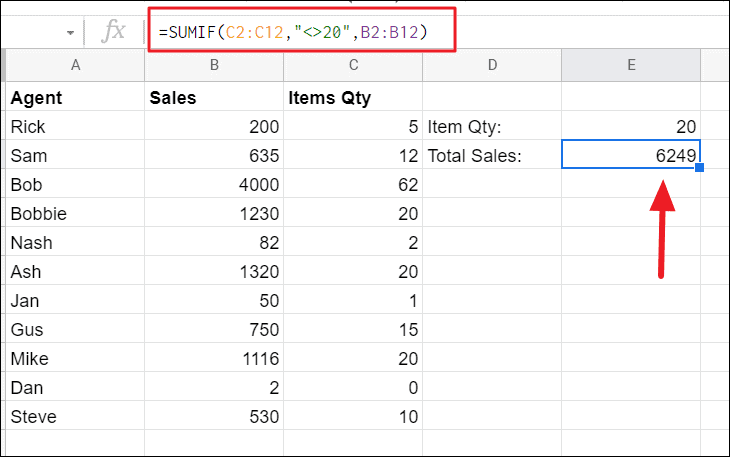
SUMIF Function with Text Criteria
If you want to add up numbers in a cell range (column or row) corresponding to the cells that have a specific text, you can simply include that text or the cell that contains the text in the criteria argument of your SUMIF formula. Please note that text string should always be enclosed in double-quotes (” “).
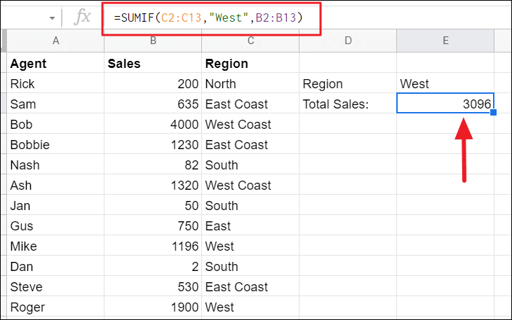
For example, if you want the total amount of sales in the ‘West’ region, you could use the below formula:
=SUMIF(C2:C13,"West",B2:B13)In this formula, the SUMIF function searches for the value ‘West’ in cell range C2:C13 and adds up corresponding sales value in column B. Then displays the result in cell E3.
You can also refer to the cell that contains text instead of using the text in the criteria argument:
=SUMIF(C2:C12,E2,B2:B12)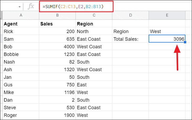
Now, let’s get the total revenue of all regions except ‘West’. To do that, we will use not equal to the operator (<>) in the formula:
=SUMIF(C2:C12,"<>"&E2,B2:B12)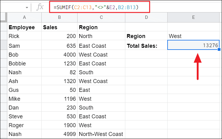
SUMIF with WildCards
In the above method, the SUMIF function with text criteria checks the range against the exact specified text. Then it sums the numbers parrel to exact text and ignores all other numbers including partially matched text string. To sum the numbers with partial matching text strings, you have to tailor one of the following wildcard characters in your criteria:
?(question mark) is used to match any single character, anywhere in the text string.*(asterisk) is used to find matching words along with any sequence of characters.~(tilde) is used to match texts with a question mark (?) or asterisk character (*).
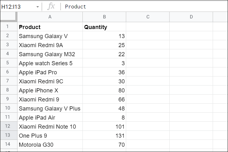
We’ll this example spreadsheet for products and their quantities to sum numbers with wildcards:
Asterisk (*) Wildcard
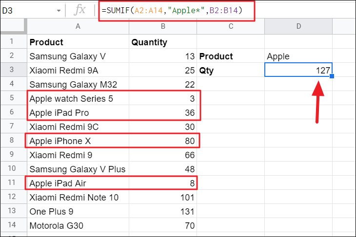
For example, if you want sum the quantities of all Apple products, use this formula:
=SUMIF(A2:A14,"Apple*",B2:B14)This SUMIF formula finds all the products with the word “Apple” at the beginning and any number of characters after it (denoted by ‘*’). Once the match is found, it sums up the Quantity numbers corresponding to the matching text strings.
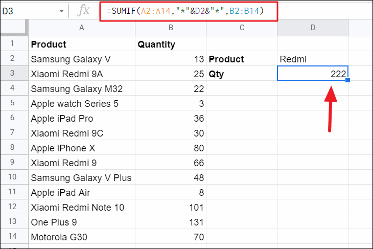
It is also possible to use multiple wildcards in the criteria. And you can also enter wildcard characters with cell references instead of direct text.
To do that, the wildcards must be enclosed in double quotation marks(“ “), and concatenated with the cell reference(s):
=SUMIF(A2:A14,"*"&D2&"*",B2:B14)This formula adds up the quantities of all the products that have the word ‘Redmi’ in them, no matter where the word is located in the string.
Question mark (?) Wildcard
You can use the question mark (?) wildcard to match text strings with any single characters.
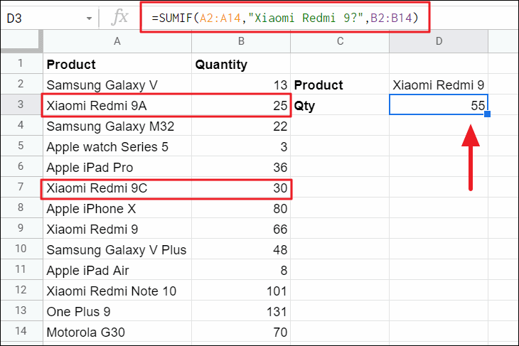
For example, if you want to find quantities of all Xiaomi Redmi 9 variants, you can use this formula:
=SUMIF(A2:A14,"Xiaomi Redmi 9?",B2:B14)The above formula looks for text strings with the word “Xiaomi Redmi 9” followed by any single characters and sums the corresponding Quantity numbers.
Tilde (~) Wildcard
If you want to match an actual question mark (?) or asterisk character (*), insert the tilde (~) character before the wildcard in the condition part of the formula.
To add the quantities in column B with the corresponding string that have an asterisk sign at the end, enter the below formula:
=SUMIF(A2:A14,"Samsung Galaxy V~*",B2:B14)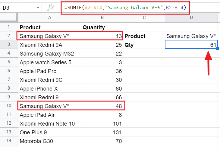
To add quantities in column B that have a question mark (?) in column A in the same row, try the below formula:
=SUMIF(A2:A14,"~?",B2:B14)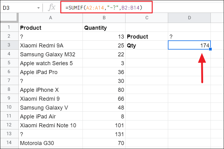
SUMIF Function with Date Criteria
SUMIF function can also help you conditionally sum values based on date criteria – for example, numbers corresponding to a certain date, or before a date, or after a date. You can also use any of the comparison operators with a date value to create date criteria for summing numbers.
The Date must be entered in Google sheets supported date format, or as a cell reference that contains a date, or using a date function such as DATE() or TODAY().
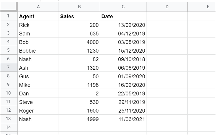
We will use this example spreadsheet to show you how SUMIF function with date criteria works:
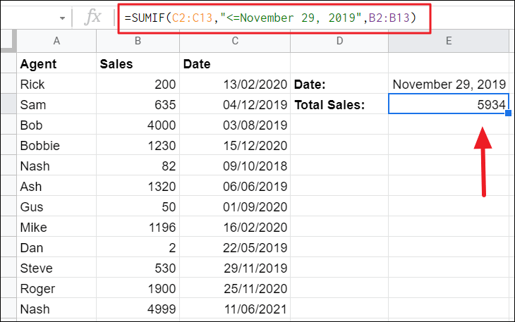
Suppose you want to sum the sales amounts that happened on or before (<=) November 29, 2019 in the above dataset, you can add those sales numbers using SUMIF function in one of these ways:
=SUMIF(C2:C13,"<=November 29, 2019",B2:B13)The above formula checks each cell from C2 to C13 and matches for only those cells that contain dates on or before November 29, 2019 (29/11/2019). And then sums the sales amount corresponding to those matching cells from the cell range B2:B13 and displays the result in cells E3.
The date can be supplied to the formula in any format that is recognized by Google Sheets, like ‘November 29, 2019′, ’29 Nov 2019′, or ’29/11/2019’, etc. Remember date value and the operator must always be enclosed in double quotation marks.
You can also use DATE() function in the criteria instead direct date vale:
=SUMIF(C2:C13,"<="&DATE(2019,11,29),B2:B13)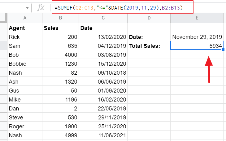
Or, you can use cell reference instead of date in the criteria part of the formula:
=SUMIF(C2:C13,"<="&E2,B2:B13)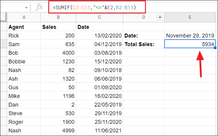
If you want to add the sales amounts together based on today’s date, you can use the TODAY() function in the criteria argument.
For example, to sum any and all sales amounts for today’s date, use this formula:
=SUMIF(C2:C13,TODAY(),B2:B13)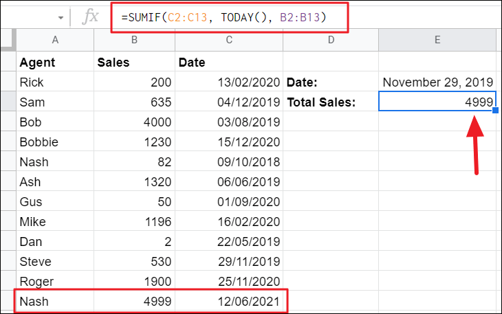
SUMIF function with Blank or Non-Blank cells
Sometimes, you may need to sum the numbers in a range of cells with blank or non-blank cells in the same row. In such cases, you can use the SUMIF function to sum values based on criteria where cells are empty or not.
Sum if Blank
There are two criterions in Google Sheets to find blank cells: “” or “=”.
For example, if you want to sum all the sales amount that contain zero-length strings (visually looks empty) in column C, use double quotation marks with no space in between in the formula:
=SUMIF(C2:C13,"",B2:B13)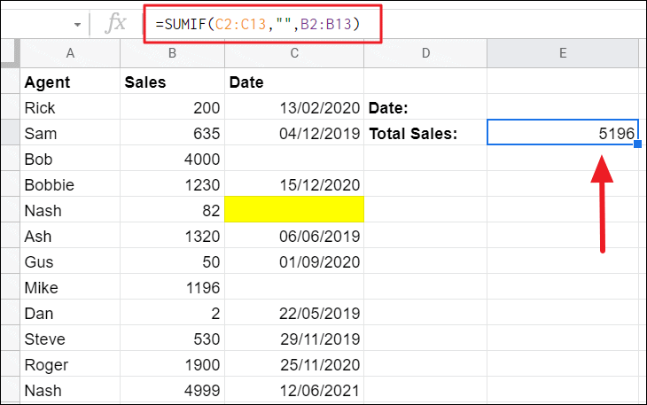
To sum all the sales amount in column B with complete blank cells in column C, include “=” as the criteria:
=SUMIF(C2:C13,"=",B2:B13)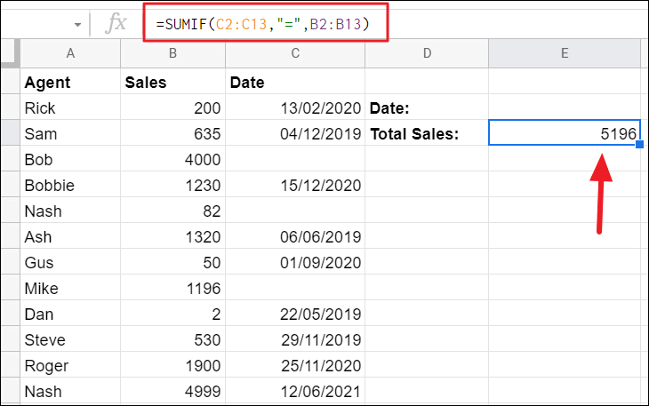
Sum if Not Blank:
If you want to sum cells that contain any value (not empty), you can use “<>” as the criteria in the formula:
For example, to get the total amount of sales with any dates, use this formula:
=SUMIF(C2:C13,"<>",B2:B13)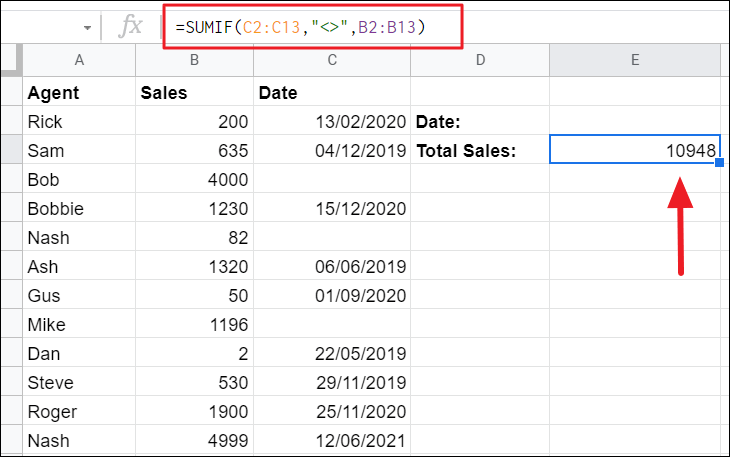
SUMIF Based on Multiple Criteria with OR Logic
As we have seen so far the SUMIF function is designed to sum numbers based on just a single criterion, but it possible to sum values based on multiple criteria with the SUMIF function in Google Sheets. It can be done by joining more than one SUMIF function in a single formula with OR logic.
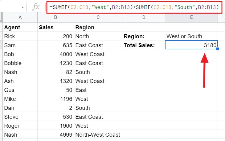
For example, if you want to sum up the sales amount in the ‘West’ region or ‘South’ region (OR logic) in the specified range (B2:B13), use this formula:
=SUMIF(C2:C13,"West",B2:B13)+SUMIF(C2:C13,"South",B2:B13)This formula sums cells when at least one of the conditions is TRUE. Hence it’s known as ‘OR logic’. It will also sum values when all conditions are met.
The first part of the formula checks the range C2:C13 for the text ‘West’ and sums the values in the range B2:B13 when the match is met. The seconds part of the checks for the text value ‘South’ in the same range C2:C13 and then sums values with the matching text in the same sum_range B2:B13. Then both sums are added together and displayed in cell E3.
In cases only one criteria is met, it will only returns that sum value.
You can also use multiple criteria instead of just one or two. And if you’re using multiple criteria, it’s better to use a cell reference as a criterion instead of writing the direct value in the formula.
=SUMIF(C2:C13,E2,B2:B13)+SUMIF(C2:C13,E3,B2:B13)+SUMIF(C2:C13,E4,B2:B13)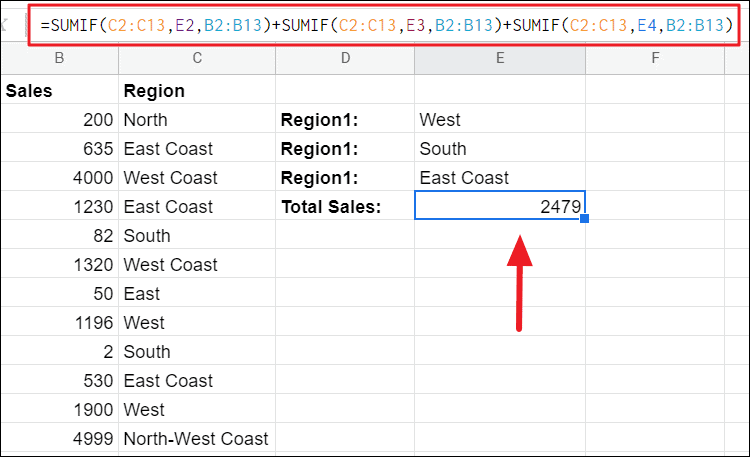
SUMIF with OR logic adds values when at least one of the specified criteria is met, But if you only want to sum values only when all the specified conditions are met, you have to use its new sibling SUMIFS() function.
SUMIFS Function in Google Sheets (Multiple Criteria)
When you use the SUMIF function to sum values based on multiple criteria, the formula may get too long and complicated, and you are prone to make mistakes. Besides SUMIF will let you sum values only on a single range and when any one of the conditions is TRUE. That’s where the SUMIFS function comes in.
The SUMIFS function helps you sum values based on multiple matching criteria in one or more ranges. And it works on AND logic, meaning it can only sum values only when all the given conditions are met. Even if one condition is false, it will return ‘0’ as a result.
SUMIFS Function Syntax and Arguments
The syntax of SUMIFS function is as follows:
=SUMIFS(sum_range, criteria_range1, criterion1, [criteria_range2, ...], [criterion2, ...])Where,
- sum_range – The range of cells containing the values you want to sum when all conditions are met.
- criteria_range1 – It is the range of cells where you check for criteria1.
- criteria1 – It is the condition which you need to check against criteria_range1.
- criteria_range2, criterion2, … – The additional ranges and criteria to evaluate. And you can add more ranges and conditions to the formula.
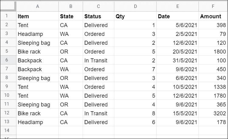
We’ll use the dataset in the following screenshot to demonstrate how the SUMIFS function works with different criteria.
SUMIFS with Text Conditions
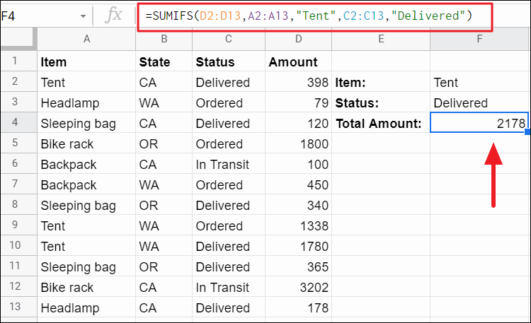
You can sum values based on two different text criteria in different ranges. For example, let’s say you want to find out the total sales amount of the delivered Tent item. For this, use this formula:
=SUMIFS(D2:D13,A2:A13,"Tent",C2:C13,"Delivered")In this formula, we have two criteria: “Tent” and “Delivered”. The SUMIFS function checks for the item ‘Tent’ (criteria1) in the range A2:A13 (criteria_range1) and checks for the status ‘Delivered’ (criteria2) in the range C2:C13 (criteria_range2). When both conditions are met, then it sums the corresponding value in the cell range D2:D13 (sum_range).
SUMIFS with Number Criteria and Logical Operators
You can use conditional operators to create conditions with numbers for the SUMIFS function.
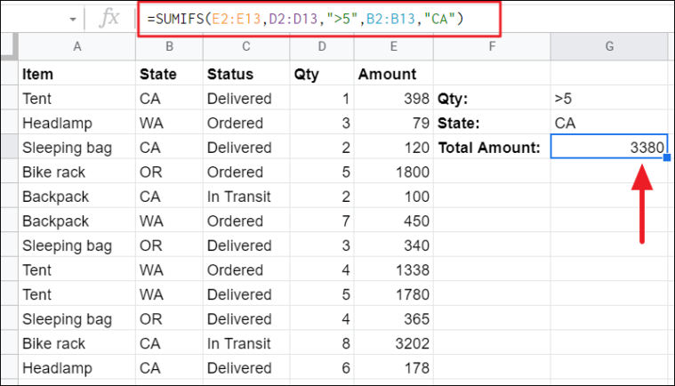
To find the total sales of more than 5 quantities of any item in the California state (CA), use this formula:
=SUMIFS(E2:E13,D2:D13,">5",B2:B13,"CA")This formula has two conditions: “>5” and “CA”.
This formula checks for quantities (Qty) greater than 5 in the range D2:D13 and checks for the state ‘CA’ in the range B2:B13. And when both conditions are met (meaning there are in the same row), it sums the amount in E2:E13.
SUMIFS with Date Criteria
SUMIFS function also allows you to check multiple conditions in the same range as well as different ranges.
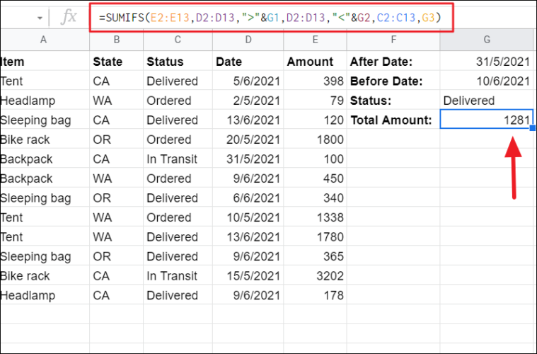
Suppose, you want to check the total sales amount of the delivered items after 31/5/2021 and before 10/6/2021 date, then use this formula:
=SUMIFS(E2:E13,D2:D13,">"&G1,D2:D13,"<"&G2,C2:C13,G3)The above formula has three conditions: 31/5/2021,10/5/2021, and Delivered. Instead of using direct date and text values, we referred to cells containing those criteria.
The formula checks for dates after 31/5/2021 (G1) and dates before 10/6/2021 (G2) in the same range D2:D13, and checks for the status ‘Delivered’ between those two dates. Then, sums the related amount in the range E2:E13.
SUMIFS with Blank and Non-Blank Cells
Sometimes, you may want to find the sum of values when a corresponding cell is empty or not. To do that, you can use one of the three criteria that we discussed before: “=”, “”, and “<>”.
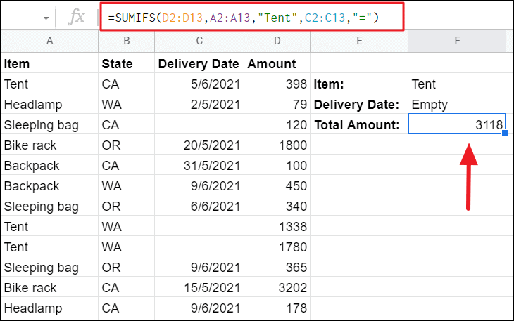
For example, if you only wish to sum the amount of ‘Tent’ items for which the delivery date has not been confirmed yet (empty cells), you could use criteria of “=”:
=SUMIFS(D2:D13,A2:A13,"Tent",C2:C13,"=")The formula looks for the ‘Tent’ item (criteria1) in column A with corresponding blanks cells (criteria2) in column C and then sums the corresponding amount in column D. The “=” represents a completely blank cell.
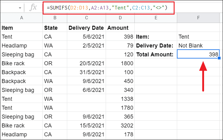
To find the sum amount of ‘Tent’ items for which the delivery date has been confirmed (not empty cells), use “<>” as a criteria:
=SUMIFS(D2:D13,A2:A13,"Tent",C2:C13,"<>")We just swapped “=” for “<>” in this formula. It finds the sum of Tent items with non-blank cells in column C.
SUMIFS with OR Logic
Since the SUMIFS function works on AND logic, it only sums when all conditions are met. But what if you want to sum value based on multiple criteria when any one of the criteria is met. The trick is to use multiple SUMIFS functions.
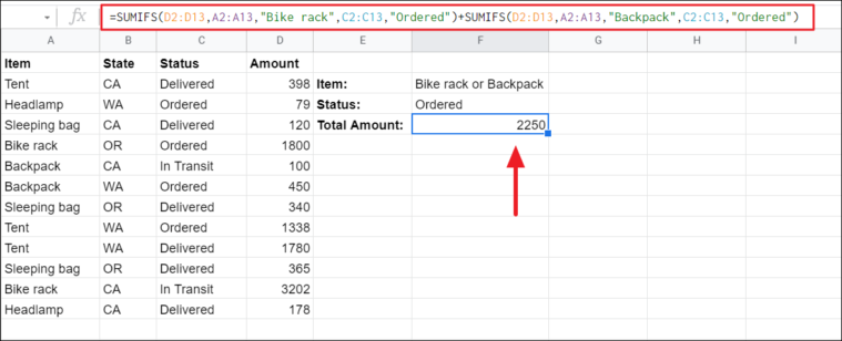
For example, if you want to add up the sales amount for either ‘Bike rack’ OR ‘Backpack’ when their status is ‘Ordered’, try this formula:
=SUMIFS(D2:D13,A2:A13,"Bike rack",C2:C13,"Ordered")
+SUMIFS(D2:D13,A2:A13,"Backpack",C2:C13,"Ordered")
The first SUMIFS function checks two criteria “Bike rack” and “Ordered” and sums the amount values in column D. Then, the second SUMIFS checks two criteria “Backpack” and “Ordered” and sums the amount values in column D. And then, both sums are added together and displayed on F3. In simple words, this formula sums when either ‘Bike rack’ or ‘Backpack’ is ordered.
That’s everything you need to know to about SUMIF and SUMIFS function in Google Sheets.