
Formatting inconsistencies in Excel workbooks often slow down data review and reduce clarity, especially when data comes from multiple sources or users. The Cell Style feature in Microsoft Excel addresses this by allowing you to apply a set of formatting options—such as font, color, number format, and borders—to cells in a single action. This not only speeds up the process but also guarantees uniformity throughout your worksheets.
Applying Built-In Cell Styles
Built-in cell styles offer a quick way to apply consistent formatting to your data. These styles group together formatting elements like font, fill color, number format, and borders, making it easy to visually organize your spreadsheet.
Step 1: Select the cells or range you want to format. This could be headers, totals, or any data that requires a specific look.
Step 2: Go to the Home tab and locate the Styles group. Click the Cell Styles dropdown arrow to open the style gallery.
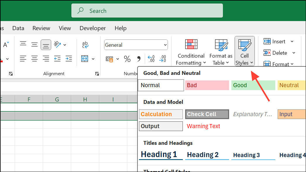
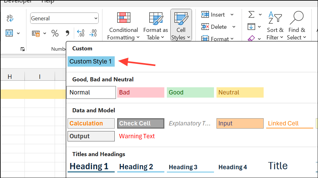
Step 3: Hover over the styles to preview how each will appear on your selected cells. Click the desired style to apply it. For example, use Heading 1 for main titles, or Good, Bad, and Neutral for quick data categorization.
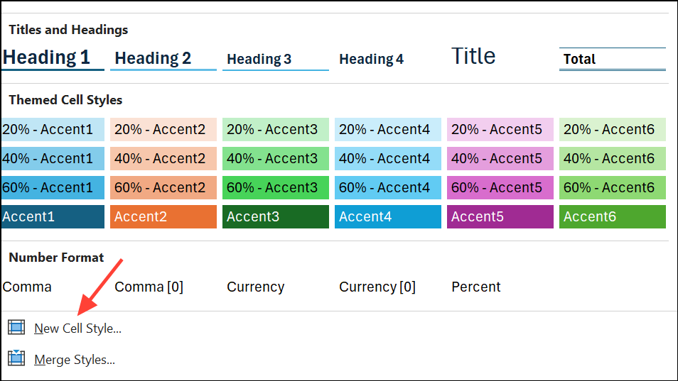
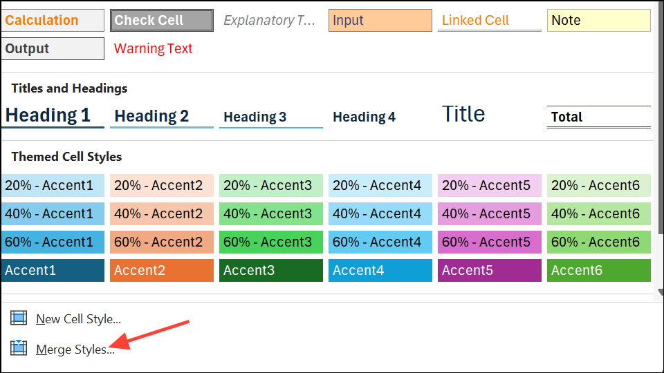
Cell styles are divided into sections like Good, Bad, and Neutral; Data and Model; Titles and Headings; Themed Cell Styles; and Number Format. These categories help you quickly find a style suitable for your data type and purpose.
Creating a Custom Cell Style
When built-in styles don't meet your needs, creating a custom cell style allows you to define exactly how your data should look and behave.
Step 1: Select a cell that already has your preferred formatting, or manually format a cell with the font, color, border, and number format you want to save as a style.
Step 2: On the Home tab, click the Cell Styles dropdown, then select New Cell Style at the bottom of the gallery.
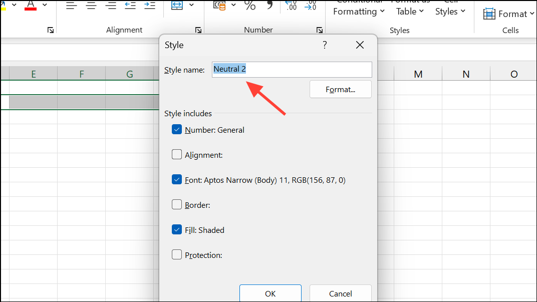
Step 3: In the dialog box, enter a descriptive name for your new style in the Style name field.
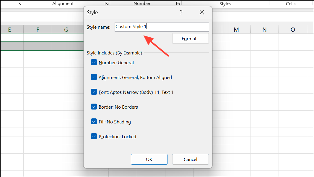
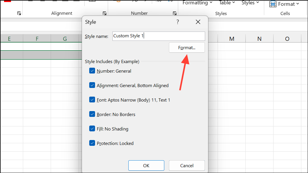
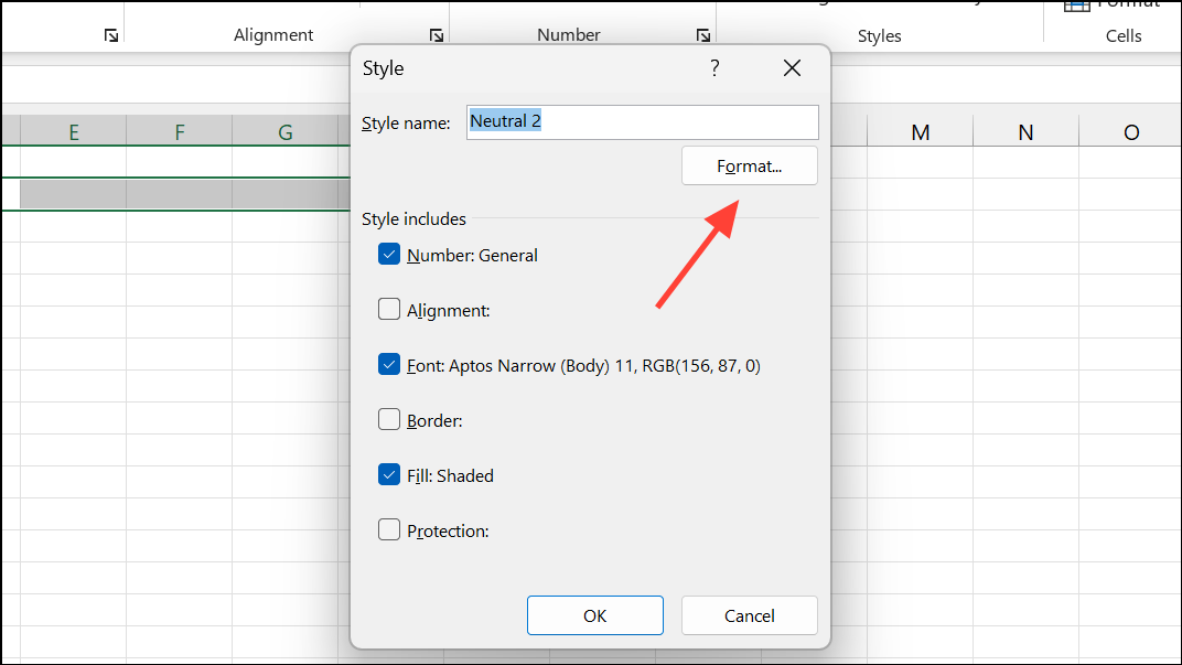
Step 4: Click Format to open the Format Cells dialog. Here, you can adjust number, alignment, font, border, fill, and protection settings. Uncheck any formatting options you don't want included.
Step 5: Click OK to save your custom style. It will now appear in the Custom section of the Cell Styles gallery for easy reuse.
Custom cell styles are especially useful for branding, recurring reports, or any scenario where a unique look is required across multiple sheets.
Modifying and Duplicating Existing Cell Styles
Adjusting an existing style or creating a variation saves time and keeps your formatting consistent. There are two main approaches:
Duplicating a Style
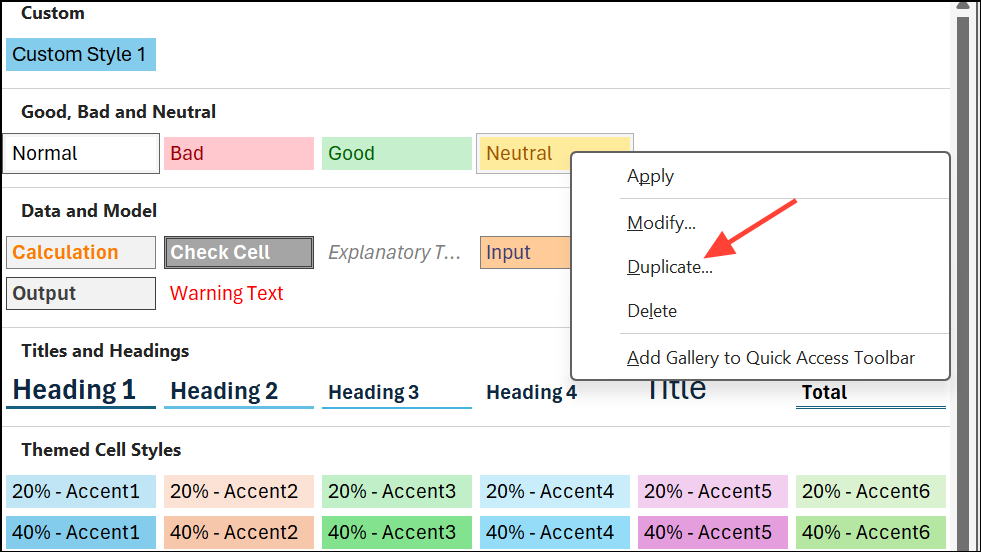
Step 1: In the Cell Styles gallery, right-click the style you want to use as a template and select Duplicate.
Step 2: Enter a new name for your duplicated style in the dialog box.
Step 3: Click Format to adjust any formatting options as needed, then click OK.
This method keeps the original style unchanged and creates a new custom style for your specific needs.
Modifying a Style
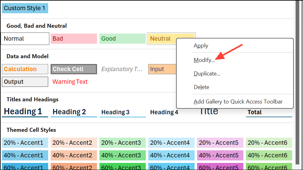
Step 1: Right-click the style you want to change and select Modify.
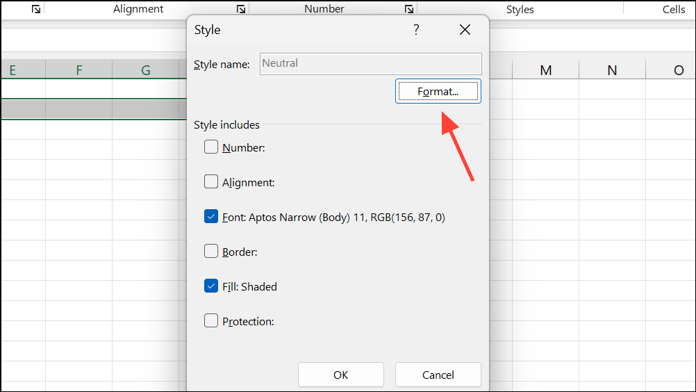
Step 2: Click Format to adjust the formatting. After making your changes, click OK.
Changes to built-in styles update all cells using that style in the workbook. Custom styles can be renamed, but built-in styles cannot.
Removing and Deleting Cell Styles
Sometimes, you may need to revert cells to their default appearance or remove unused styles from your workbook.
Removing a Cell Style from Data
Step 1: Select the cells currently formatted with a style you want to remove.
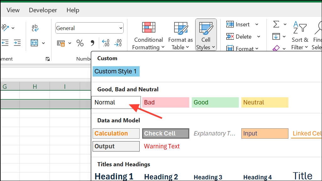
Step 2: Open the Cell Styles gallery and click Normal under the Good, Bad, and Neutral section. This resets selected cells to Excel's default formatting.
Deleting a Cell Style
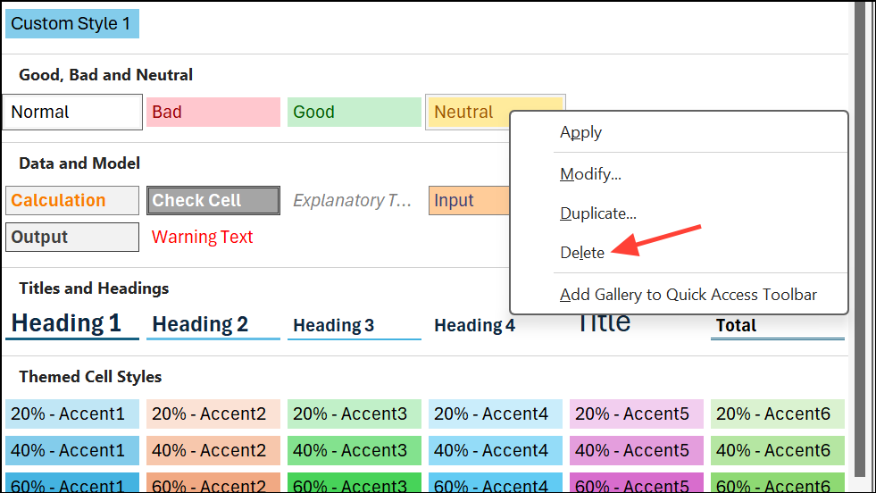
Step 1: In the Cell Styles gallery, right-click the custom or predefined style you want to delete and choose Delete.
Deleting a style removes it from all cells using it in your workbook.
Normal style cannot be deleted.Copying Cell Styles Between Workbooks
To maintain consistency across multiple workbooks, you can import cell styles from one file to another using the Merge Styles feature.
Step 1: Open both the source workbook (with the styles you want) and the destination workbook.
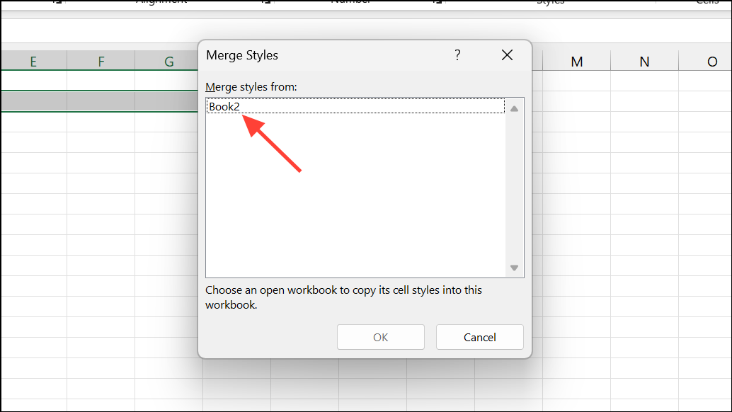
Step 2: In the destination workbook, go to the Home tab, click Cell Styles, and then select Merge Styles at the bottom of the dropdown menu.
Step 3: Choose the source workbook in the dialog box and click OK. The imported styles will now be available in your destination workbook.
This process is especially useful for applying consistent branding or formatting standards across multiple projects, or for restoring deleted built-in styles.
Making Cell Styles Available in All New Workbooks
If you want your custom cell styles to be readily available every time you create a new workbook, you can save them in a template file.
Step 1: Create a new workbook and set up your custom cell styles as needed.
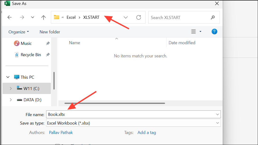
Step 2: Save the workbook as Book.xltx in your Excel startup folder, typically located at %appdata%\Microsoft\Excel\XLSTART. You can access this hidden folder by entering %appdata% in the File Explorer address bar and navigating to Microsoft > Excel > XLSTART.
Step 3: After saving, any new workbook you create (using Ctrl+N or the New command) will include your custom styles by default. Existing workbooks will not be affected.
This approach streamlines formatting in future workbooks and eliminates the need to manually recreate styles each time.
Using the Cell Style feature in Excel speeds up formatting, keeps your data visually consistent, and reduces repetitive manual work. Whether you're managing reports, financial statements, or project trackers, mastering cell styles can save you time and improve the clarity of your spreadsheets.