
The TREND function in Excel can help you find out the line of best fit from the data present in a chart with the help of the least-squares statistical method. The equation to calculate it is y = mx + b. Here y stands for the dependent variable, m is the steepness or gradient of the line, x stands for the independent variable, and b is the point where the trendline and the y-axis intercept.
Using the TREND function
You can use the TREND function in several instances, such as when you have the revenue for a specific time period and want to find out the trend for that data.
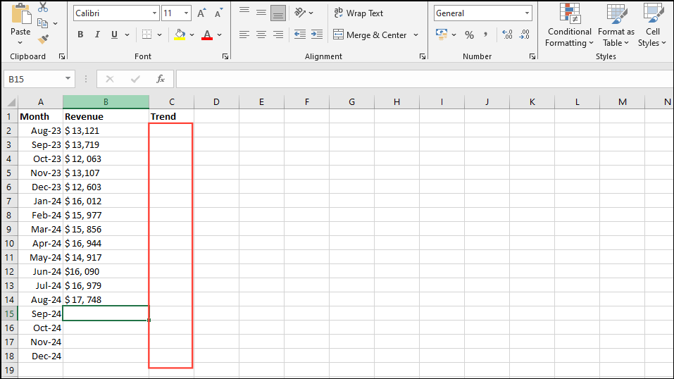
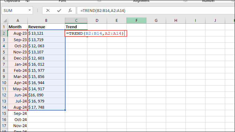
- For the example shown above, type the following formula in cell C2:
=TREND(B2:B14,A2:A14). Here, 'B2:B14' are known y-values while 'A2:A14' are known x-values.
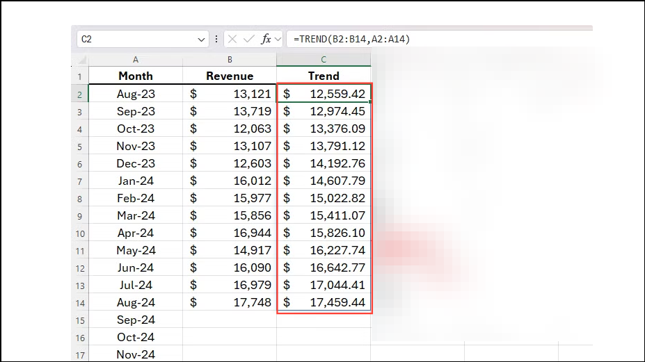
- Press Enter after entering the formula and you will see the trend displayed in the form of an array.
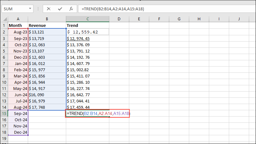
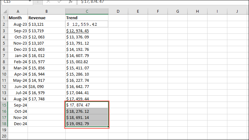
- Once you have the trend, you can use the data to get information for the remaining period. Type
=TREND(B2:B14,A2:A14,A15:A18)in Cell 15C. Here, 'A2:A14' are known x-values while 'B2:B14' are known y-values.
- Press Enter to get the values for the remaining period.
TREND function in charts
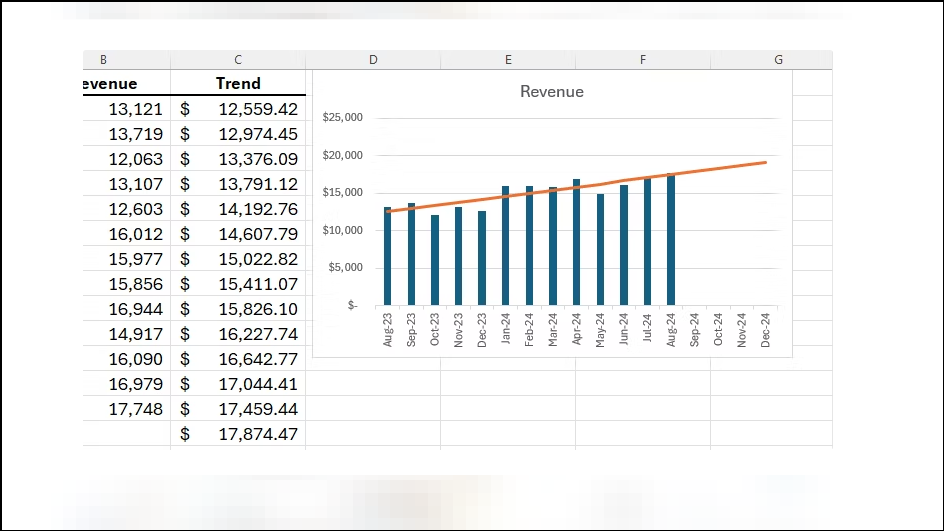
Once you have obtained the data using the TREND function, you can view it in chart form.
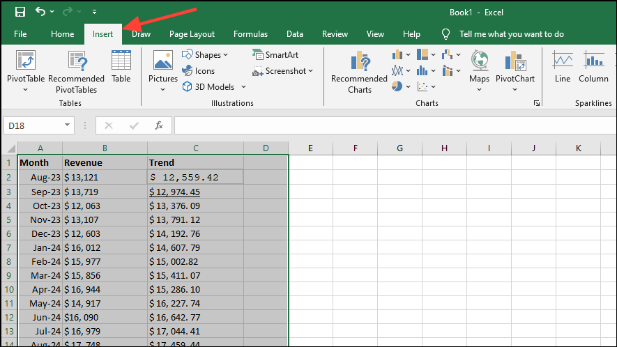
- Select all the data in your worksheet along with the headings and click on the 'Insert' tab at the top.
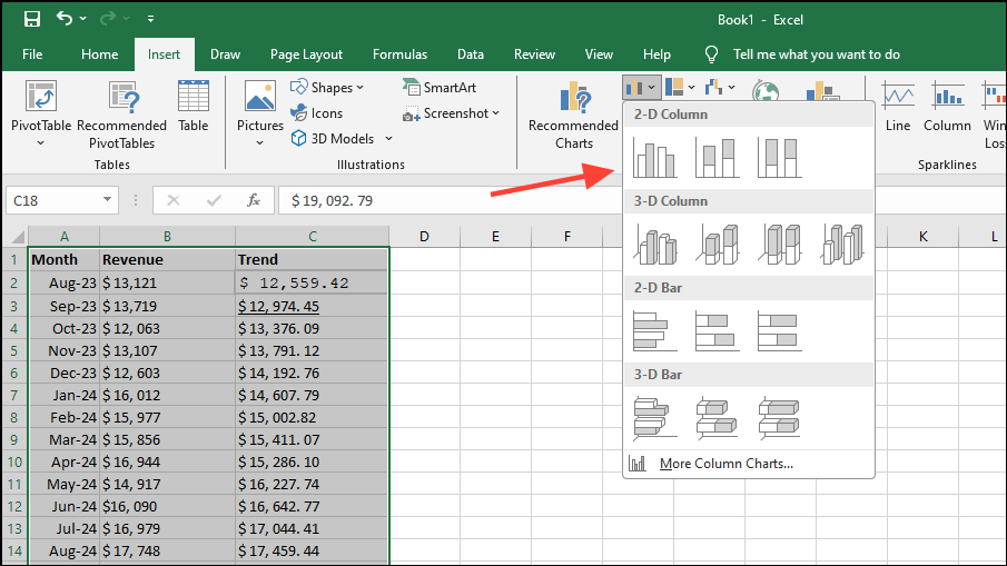
- Then click on '2D Clustered Column Chart' from the charts option. The option may appear differently depending on your version of Excel.
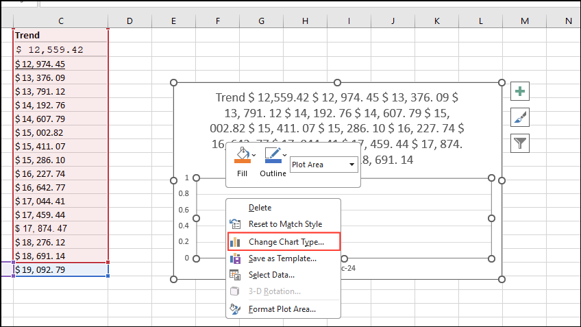
- When you insert the chart, the data will show both the revenue (independent variable) and the trendline. To view the trend as a line, right-click anywhere on the chart and click on 'Change chart type'.
- Then click on 'Combo' from the options. Check the trendline option is set to 'Line'.
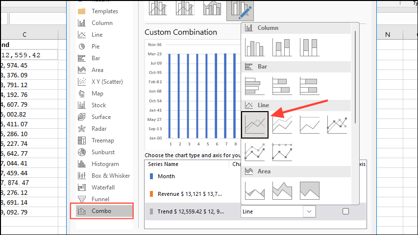
- Click on the 'OK' button and the new chart will appear. If you want, you can click on the '+' icon in the corner which will get rid of the legend.
After creating and visualizing the trend of your data, you can calculate its slope.
Note: You can also calculate the slope of your data in Excel using the
=SLOPE(known_Ys, knownXs) formula. Select the cell where you want the output to appear, then enter the formula with the cell range. When you press Enter, Excel will show you the slope indicating the rate of change in the data.Things to know
- The TREND function uses a similar algorithm to the FORECAST function but it analyzes past data while the latter predicts the future performance of a series.
- You can also add a trendline to a chart in Excel without using the TREND function if you do not want it to show future predictions.
- Sparklines are another Excel feature found in the 'Insert' tab which can also help you see trends in your data.
- If you use formulas that provide information in the form of arrays, you need to enter them as array formulas using
Ctrl + Shift + Enter. However, if you are using a current version of Microsoft 365, just press Enter.