Whenever you enter or import numbers with one or more leading zeros, like 000652, Excel automatically removes those zeros, and only the number itself shows in the cells (652). This is because the leading zeros are not necessary for calculations and do not count.
However, there are times when those leading zeros are necessary, like when you’re entering ID numbers, phone numbers, credit card numbers, product codes, or postal codes, etc. Fortunately, Excel gives us several ways to add or keep leading zeros in cells. In this article, We will show you the different ways to add or keep leading zeros and remove leading zeros.
Adding Leading Zeros in Excel
Essentially, there are 2 methods that you can use to add leading zeros: one, format your number as ‘Text’; two, use custom formatting to add leading zeros. The method you want to use may depend on what you want to do with the number.
You may want to add leading zero when you are entering unique ID numbers, account numbers, social security numbers, or zip codes, etc. But, you are not going to use these numbers for calculations or in functions, so it best to convert those numbers to text. You would never sum or average phone numbers or account numbers.
There are several ways you can add or pad zeros before the numbers by formatting them as text:
- Changing the cell format to Text
- Adding an apostrophe (‘)
- Using TEXT function
- Using REPT/LEN Function
- Use CONCATENATE Function/Ampersand operator (&)
- Using RIGHT function
Changing the Cell Format to Text
This is one of the simplest ways to add leading zeros to your numbers. If you are just going to enter numbers and you want to keep leading zeros as you type, then this is the method for you. By changing cell format from General or Number to Text, you can force Excel to treat your numbers as text values and anything you type in the cell will stay exactly the same. Here’s how you do it:
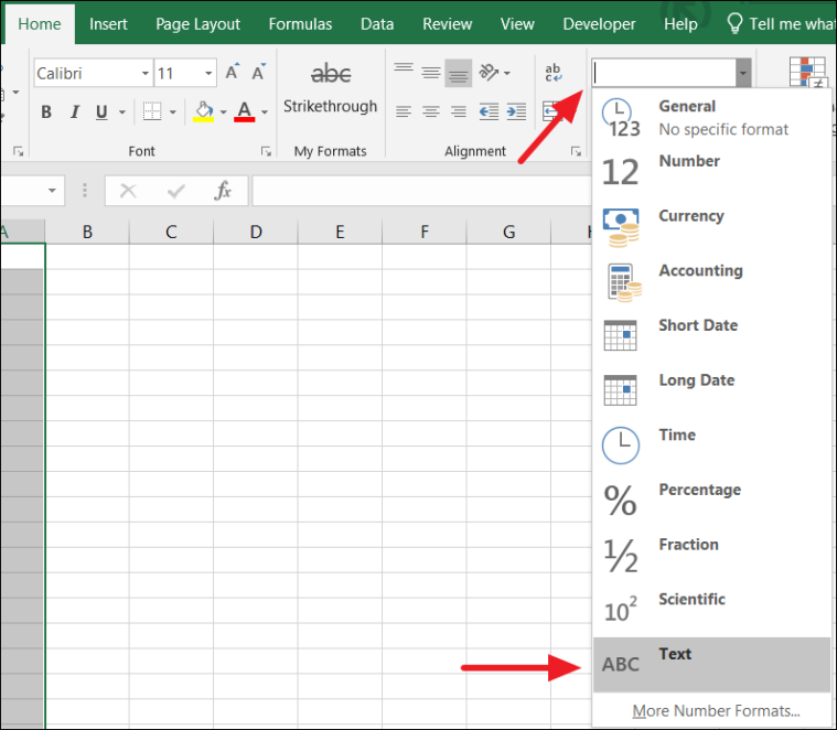
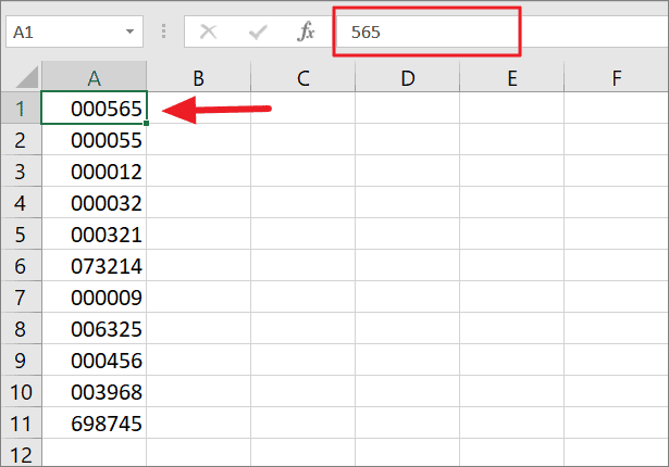
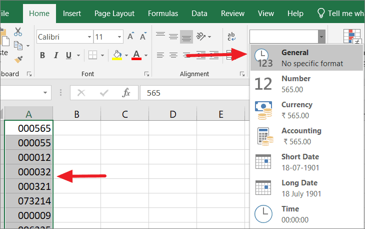
Select the cell(s) in which you want to add leading zeroes. Go to the ‘Home’ tab, click on the ‘Format’ drop-down box in the Numbers group, and select ‘Text’ from the format options.
Now when you type your numbers, Excel will not delete any leading zero from it.
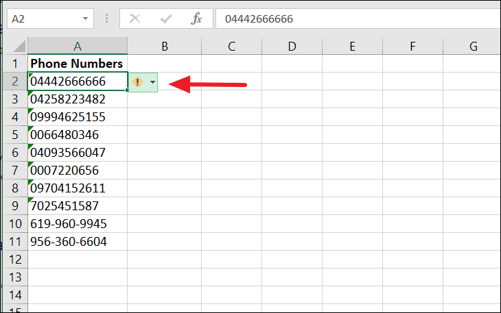
You might see a small green triangle (Error indicator) in the top-left corner of the cell and when you select that cell, it will show you a warning sign indicating that you have stored the number as text.
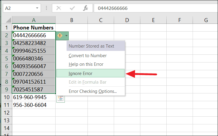
To remove the error message, select the cell(s), click on the warning sign, and then select ‘Ignore Error’ from the list.
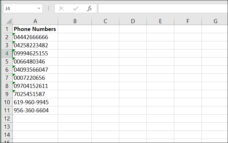
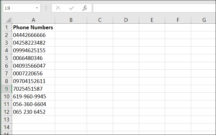
You can also type phone numbers with space or hyphen between number, Excel will automatically treat these numbers as text.
Using Leading Apostrophe ( ‘ )
Another way to add leading zeros in Excel is to add an apostrophe (‘) at the start of the number. This will force Excel to enter a number as text.
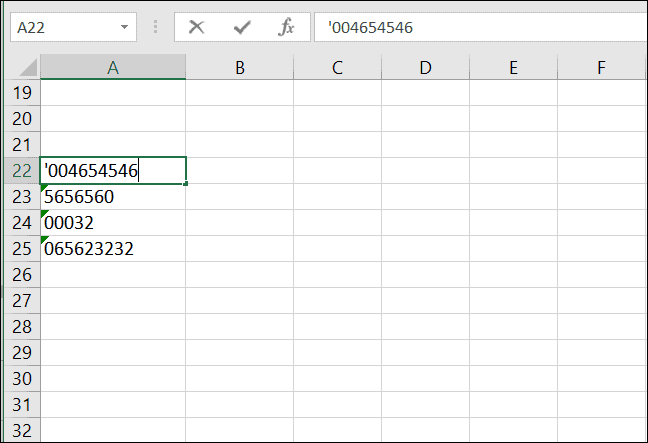
Just type an apostrophe before any numbers and hit ‘Enter’. Excel will leave the leading zeros intact, but the (‘) will not be visible in the worksheet not unless you select the cell.
Using Text Function
The above method adds zeros to numbers as you type them, but if you already have a list of numbers and you want to pad leading zeros before them, then the TEXT function is the right method for you. TEXT function allows you to convert numbers to text strings while applying custom formatting.
The Syntax of TEXT function:
= TEXT( value, format_text)Where,
- value – It is the numerical value that you need to convert to text and apply formatting.
- format_text – is the format you want to apply.
With the TEXT function, you can specify how many digits your number should have. For example, if you want your numbers to be 8 digits long, then type 8 zeros in the second argument of function: “00000000”. If you have 6 digit number in a cell, then the function will manually add 2 leading zeros and if you have 2 digit numbers like 56, the rest will be zeros (00000056).
For example, to add leading zeros and make the numbers 6-digit long, use this formula:
=TEXT(A2,"000000")Since we have 6 zeros in the second argument of the formula, the function converts the number string into a text string and adds 5 leading zeros to make the string 6 digits long.
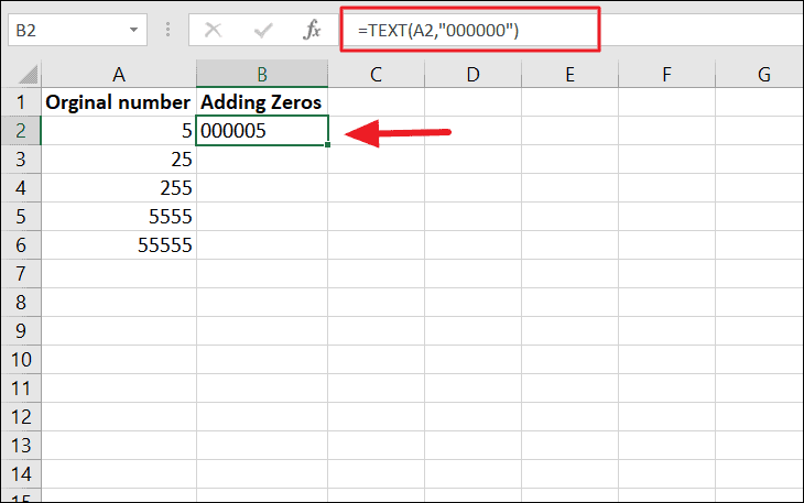
Note: Please remember to enclose the format codes in double quotation marks in the function.
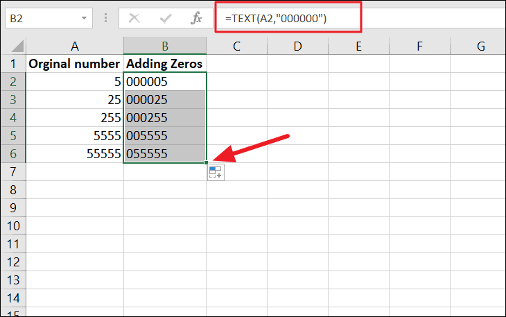
Now you can apply the same formula to the rest of the cells by dragging the fill handle. As you can see, the function converts the numbers into texts and add leading zeros to the numbers so that the total number of digits is 6.
TEXT Function will always return value as a text string, not a number, so you won’t be able to use them in arithmetic calculations but you can still use them in lookup formulas such as VLOOKUP or INDEX/MATCH to fetch the details of a product using Product IDs.
Using CONCATENATE Function/Ampersand Operator (&)
If you want to add a fixed number of leading zeros before all numbers in a column, you can use CONCATENATE function or the ampersand operator (&).
Syntax of CONCATENATE function:
=CONCATENATE(text1, [text2], ...)Where,
text1 – The number of zeros to be inserted before the number.
text2 – The original number or cell reference
Syntax of Ampersand operator:
=Value_1 & Value_2 Where,
Value_1 is the leading zeros to insert before the number and Value_2 is the number.
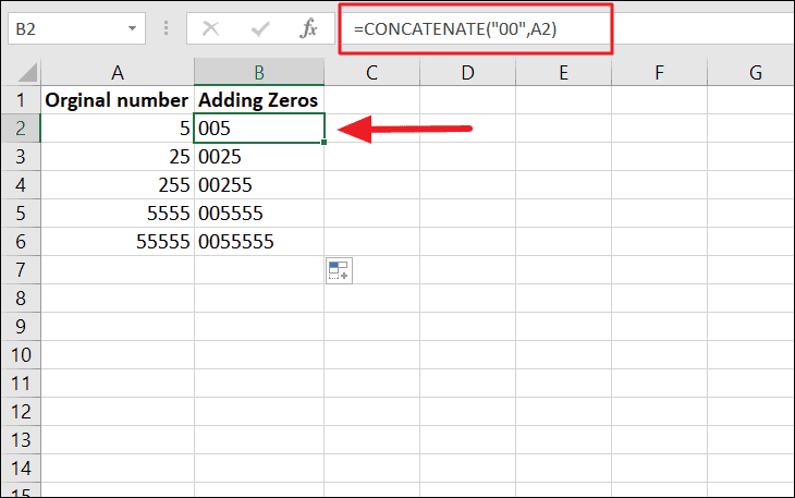
For example, to add only two zeros before a number, use either of this formula:
=CONCATENATE("00",A2)The first argument is two zeros (“00”) because we want to pad two zeros before the number in A2 (which is the second argument).
Or,
="00"&A2Here, the first argument is 2 zeros, followed by ‘&’ operator, and the second argument is the number.
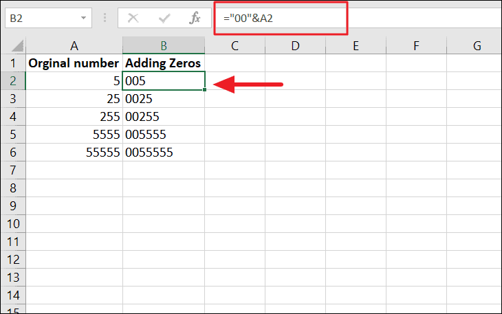
As you can see the formula adds just two leading zeros to all the numbers in a column regardless of how many digits the number contains.
Both of these formulas join a certain number of zeros before the original numbers and stores them as text strings.
Using REPT/LEN Function
If you want to add leading zeros to numeric or alphanumeric data and convert the string into text, then use the REPT function. The REPT function is used to repeat a character(s) a specific number of times. This function can also be used to insert fixed numbers of leading zeros before the number.
=REPT(text, number_times)Where ‘text’ is the character we want to repeat (in our case ‘0’) and ‘number_times’ argument is the number of times we want to repeat that character.
For example, to generate five zeros before numbers, the formula would look like:
=REPT(0,5)&A2What the formula does is repeat 5 zeros and joins the number string in A2 and returns the result. Then, the formula is applied to cell B2:B6 using the fill handle.
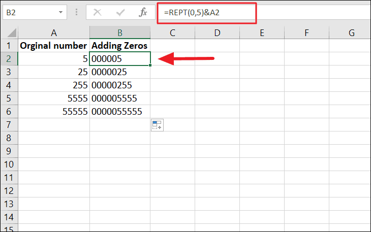
The above formula adds a fixed number of zeros before the number, but the total length of the number varies depending on the number.
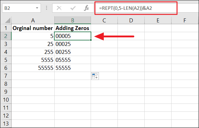
If you want to add leading zeroes wherever needed to create a specific character long (fixed length) strings, you can use REPT and LEN functions together.
Syntax:
=REPT(text, number_times-LEN(text))&cellFor example, to add prefixed zeroes to the value in A2 and make a 5-character long string, try this formula:
=REPT(0,5-LEN(A2))&A2Here, ‘LEN(A2)’ gets total the length of the string/numbers in cell A2. ‘5’ is the maximum length of string/numbers the cell should have. And ‘REPT(0,5-LEN(A2))’ part adds the number of zeros by subtracting the length of the string in A2 from the maximum number of zeros (5). Then, a number of 0’s is joined before the value of A2 to make a fixed-length string.
Using RIGHT Function
Another way to pad leading zeros before a string in Excel is use the RIGHT function.
The RIGHT function can add a number of zeros to the start of a number and extract the right-most N characters from the value.
Syntax:
= RIGHT (text, num_chars)- text is the cell or value you want to extract characters from.
- num_chars is the number of characters to extract from the text. If this argument is not given, then only the first character will be extracted.
For this method, we concatenating the maximum number of zeros with cell reference that contains the string in the ‘text’ argument.
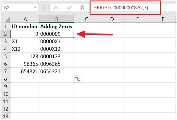
To create a 6-digit number based on the number string in A with leading zeros, try this formula:
=RIGHT("0000000"&A2,6)The first argument (text) of the formula adds 7 zeros to the value in A2 (“0000000”&A2), and then returns the rightmost 7 characters, which results in some leading zeros.
Adding Leading Zeroes using Custom Number Formatting
If you use any of the above methods to put leading zeros before the numbers, you will always get a text string, not a number. And they won’t be much use in calculations or in numeric formulas.
The best way to add leading zeros in Excel is to apply a custom number formatting. If you add leading zeros by adding a custom number format to the cell, it doesn’t change the value of the cell but only the way it is displayed. The value will still remain as a number, not text.
To change the number formatting of cells, follow these steps:
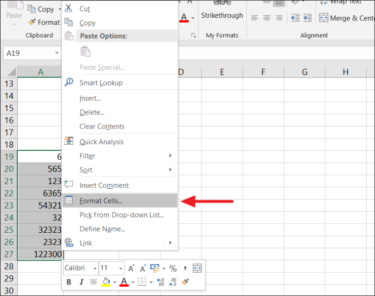
Select the cell or range of cells where you want to show leading zeros. Then, right-click anywhere within that selected range and select the ‘Format Cells’ option from the context menu. Or press the shortcut keys Ctrl + 1.
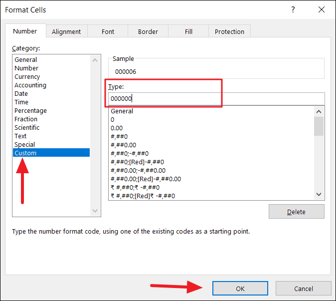
In the Format Cells window, go to the ‘Number’ tab and select ‘Custom’ under the Category options.
Enter the number of zeros in the ‘Type:’ box to specify the total number of digits you want to show in a cell. For example, if you want the number to be 6 digits long, then enter ‘000000’ as the custom format code. Then, click ‘OK’ to apply.
This will show leading zeros before the numbers and if the number is less than 6 digits, it pads zero before it.
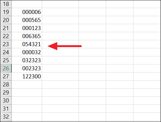
Numbers will only appear to have leading zeros while the underlying value would remain unchanged. If you select a cell with custom formatting, it will show you the original number in the formula bar
There are a lot of digital placeholders you can use in your custom number format. But there are only two primary placeholders you can use for adding leading zeros in numbers.
- 0 – It is the digit placeholder that displays extra zeros. It displays forced digits 0-9 whether or not the digit is relevant to the value. For example, if you type 2.5 with the format code 000.00, it will display 002.50.
- # – It is the digit placeholder that displays optional digits and does not include extra zeros. For example, if you type 123 with the formatting code 000#, it will display 0123.
Also, any punctuation mark or other character you include in the format code will be displayed as it is. You can use characters like hyphen (-), comma (,), forward-slash (/), etc.
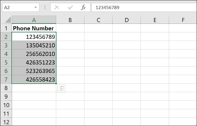
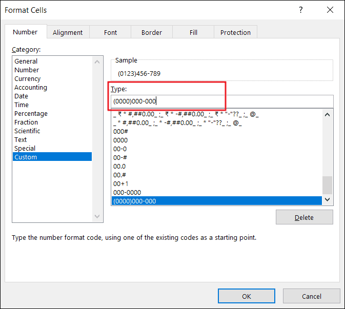
For example, you can also format numbers as phone numbers by using custom format.
The Format code in Format Cells dialog box:
The result:
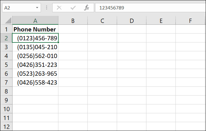
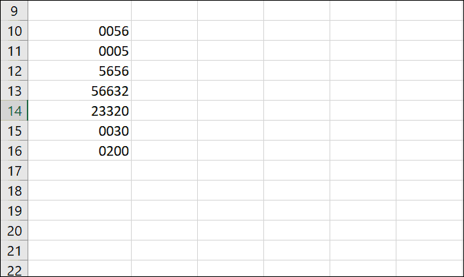
Let’s apply this formatting code in the following example:
##0000
As you can see ‘0’ will add extra zeros while ‘#’ doesn’t add insignificant zeros:
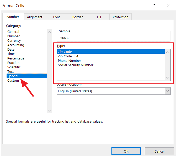
You can also use predefined format codes in the ‘Special formats’ section of the Format cells dialog box for postal codes, telephone numbers, and social security numbers.
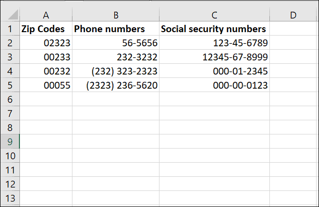
The following table shows numbers with leading zeros where different ‘Special’ format codes are applied to different columns:
Removing Leading Zeros in Excel
Now, you have learned how to add leading zeros in Excel, let’s see how to remove the leading zeros from the number of strings. Sometimes, when you import data from an external source, numbers may end up having prefix zeros and being formatted as text. In such cases, you need to remove the leading zeros and convert them back to numbers, so you can use them in formulas.
There are various ways you can remove leading zeros in Excel and we’ll see them one by one.
Remove Leading Zeros by Changing the Cell Formatting
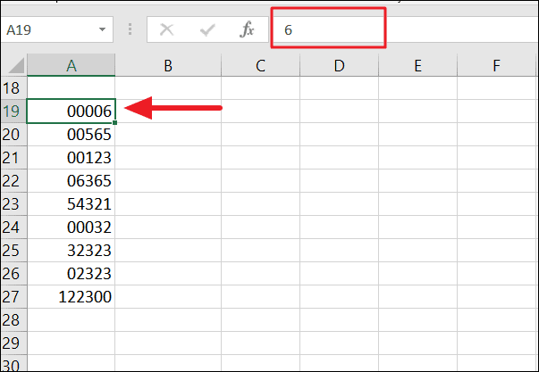
If leading zeros were added by custom number formatting, then you can easily remove them by changing the format of the cells. You can tell if your cells are custom formatted by looking at the address bar (zeros will be visible in the cell not in the address bar).
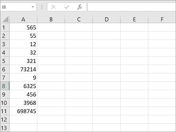
To remove the prefixed zeros, select the cells with the leading zeros, click on the ‘Number Format’ box, and select ‘General’ or ‘Number’ formatting option.
Now, the leading zeros are gone:
Delete Leading Zeros by Converting the Text to Numbers
If your leading zeros were added by changing the cell format or by adding apostrophes before the numbers or automatically added when importing data, the easiest way to convert them to numbers is by using the Error Checking Option. Here’s how you do it:
You can use this method if your numbers are left-aligned and your cells have a little green triangle (An error indicator) in the top-left corner of the cells. This means the numbers are formatted as text.
Select those cells and you will see a yellow warning at the top right part of the selection. Then, click the ‘Convert to Number’ option from the drop-down.
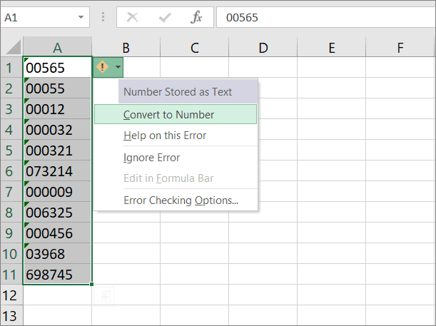
Your zeros will be removed and the numbers will be converted back to the number format (Right-aligned).
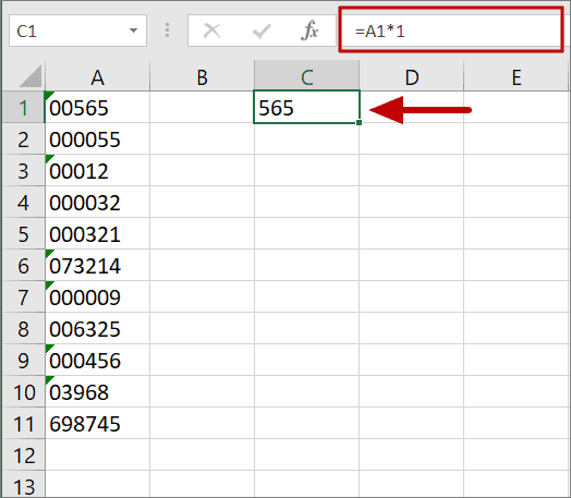
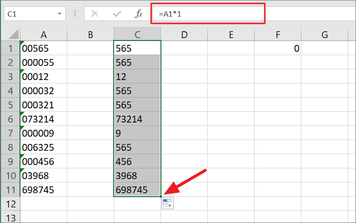
Removing Leading Zeros by Multiply/Dividing by 1
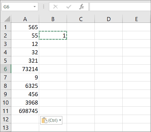
Another easy and best way to remove leading is by multiplying or dividing the numbers with 1. Dividing or multiplying the value doesn’t change the value, it simply converts the value back to a number and removes the leading zeros.
To do this, type the formula in the below example in a cell and press ENTER. The leading zeros will be removed and the string will be converted back to a number.
Then, apply this formula to other cells using the fill handle.
You can achieve the same results by using ‘Paste Special’ Command. Here’s how:
Type ‘1’ numeric value in a cell (lets say in B2) and copy that value.
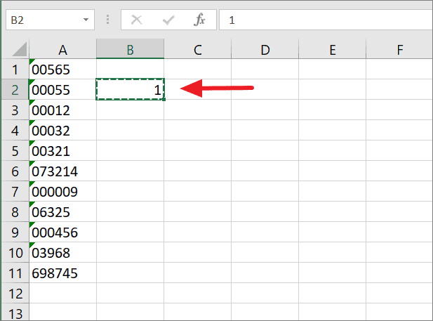
Next, select the cells in which you want to remove the leading zeros. Then, right-click on the selection and then select the ‘Paste Special’ option.
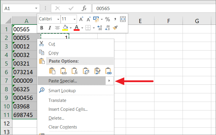
In the Paste Special dialog box, under Operation, choose either the ‘Multiply’ or ‘Divide’ option and click ‘OK’.
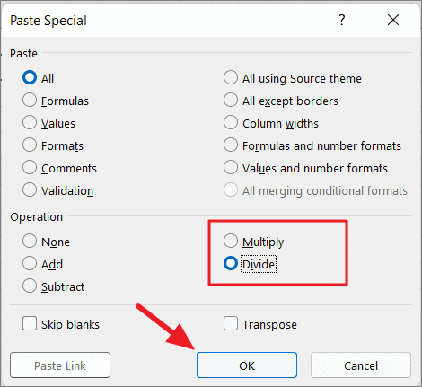
That’s it, your leading zeros will be removed leaving the strings as numbers.
Remove Leading Zeros by using a Formulas
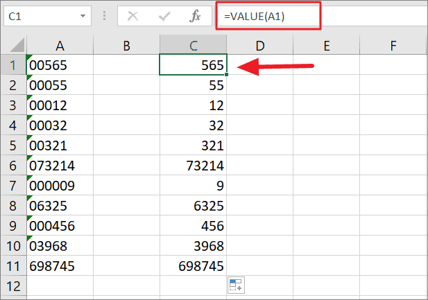
Another easy way to delete prefixed zeros is by using the VALUE function. This method could be useful whether your leading zeros were added by using another formula or apostrophe or by custom formatting.
=VALUE(A1)The argument of the formula could be a value or the cell reference that has the value. The formula removes the leading zeros and converts the value from text to number. Then apply the formula to the rest of the cells.
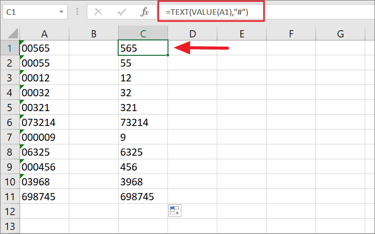
Sometimes, you may want to remove the leading zeros but want to keep the numbers in the text format. In such cases, you have to use TEXT() and VALUE () functions together like this:
=TEXT(VALUE(A1),"#")The VALUE function converts the value in A1 to number. But the second argument, ‘#’ converts the value back to text format without any extra zeros. As a result, you would get the numbers without any leading zeros but still in the text format (left-aligned).
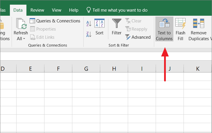
Remove Leading Zeros using Excel’s Text to Columns Feature
Yet another way to remove leading zeros is to use Excel’s Text to Columns feature.
Select the range of cells that have the numbers with leading zeros.
Next, go to the ‘Data’ tab and click on the ‘Text to Columns’ button in the Data Tools group.
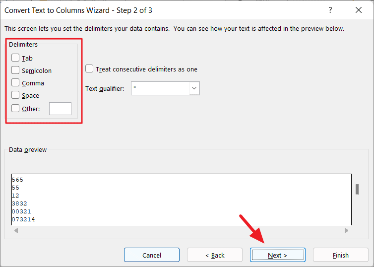
The ‘Convert Text to Columns’ wizard will appear. In step 1 of 3, select ‘Delimited’ and click ‘Next’.
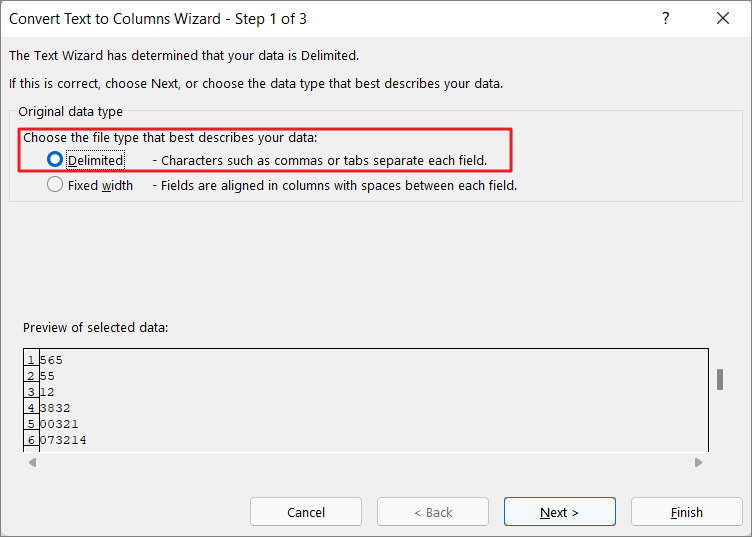
In step 2 of 3, uncheck all the delimiter and click ‘Next’.
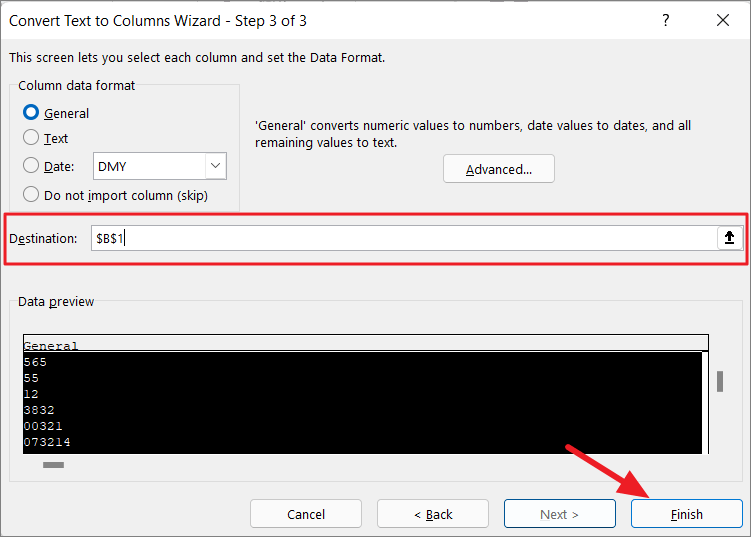
On the final step, leave the Column data format option as ‘General’ and choose the destination (the first cell of the range) where you want your numbers without leading zeros. Then, click ‘Finish’
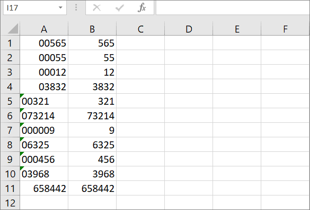
And you will get the numbers with leading removed in a separate column as shown below.
That is all.


