
Microsoft Excel is a versatile tool for managing various types of data, including financial records, sales figures, customer details, and more. Organizing data alphabetically in worksheets enhances accessibility and reference efficiency. In Excel, alphabetizing involves sorting a range of cells in alphabetical order, either ascending (A to Z) or descending (Z to A).
For example, consider a large dataset containing customer order information. Locating a specific customer’s order history manually can be time-consuming. By alphabetizing the relevant columns, you can quickly find the necessary data without extensive searching.
Excel offers multiple methods to alphabetize data, catering to different dataset types. You can sort individual columns or rows, selected ranges, or entire worksheets. Additionally, Excel provides options to group multiple columns or rows together during the sorting process. Below, we explore various techniques to alphabetize data in Excel spreadsheets by rows or columns.
Benefits of Alphabetizing Data in Excel
Sorting data alphabetically in Excel provides numerous advantages:
- Enhances data readability and organization.
- Facilitates easy lookup of specific values or customer names.
- Helps identify duplicate records, reducing data entry errors.
- Allows grouping of columns or lists for side-by-side comparison.
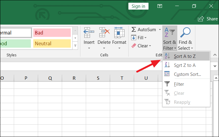
Alphabetizing is a simple yet powerful way to organize information, especially in large datasets. The primary methods to alphabetize data in Excel include using the A-Z or Z-A buttons, the Sort feature, the Filter function, and formulas.
Alphabetizing a Column in Excel
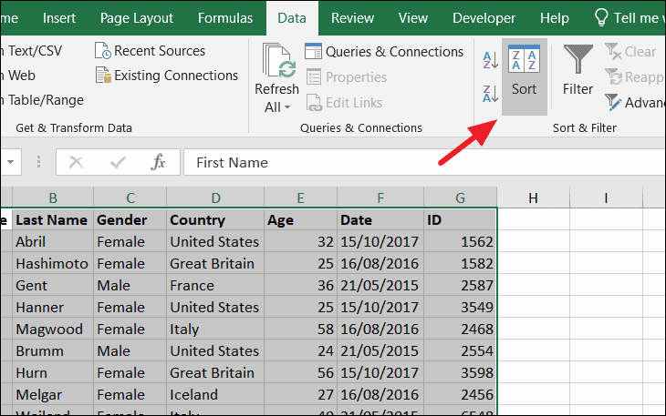
The quickest method to alphabetize a column is by utilizing Excel’s built-in Sort feature.
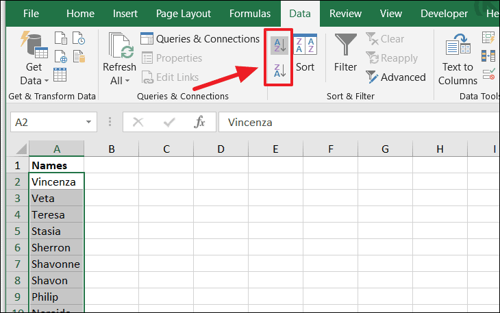
Note: If there are blank cells within your selection, Excel may only sort the data up to the first blank cell. To sort the entire column without selecting specific cells, you can simply select any single cell within the column and apply the sorting option.
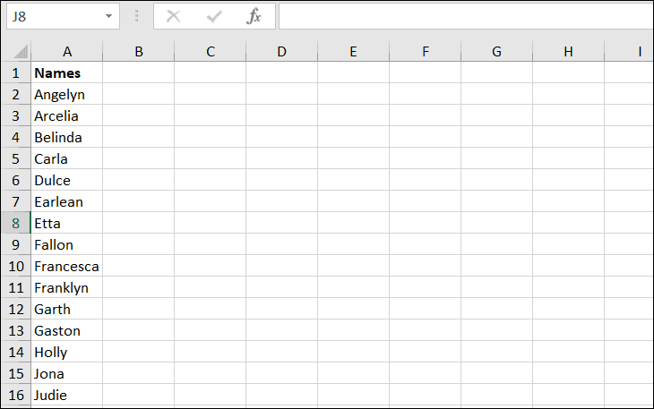
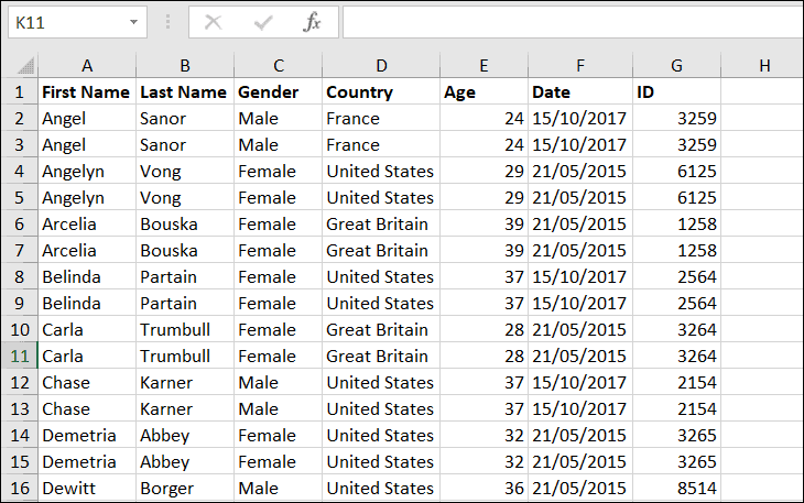
Once the sorting option is applied, Excel will immediately alphabetize your list.
Sorting and Keeping Rows Together
When working with a worksheet containing multiple columns, it’s crucial to keep rows intact during the sorting process to prevent data from mismatching. For instance, if you’re sorting a list of student names alphabetically, you want their corresponding marks or information in adjacent columns to stay correctly aligned.
Upon initiating the sort, a Sort Warning dialog box may appear. Choose the option Expand the selection and click Sort.
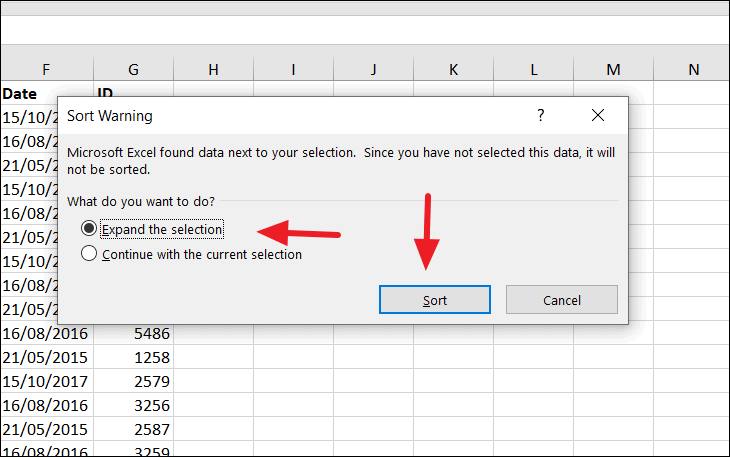
This ensures that all the data in the rows remain together, preserving the relationships between columns.
If you choose Continue with the current selection, only the selected column will be sorted, which may result in data misalignment.
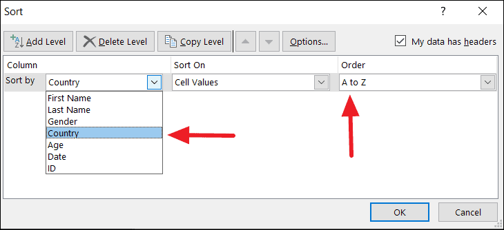
Sorting Alphabetically by Multiple Columns
Excel allows you to sort data alphabetically using multiple columns as criteria. This is useful when you need to organize data based on more than one category.
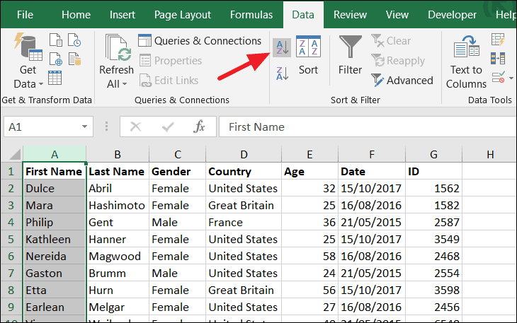
For example, suppose you have a table with columns for Country and First Name, and you want to sort the data first by country and then by first name.
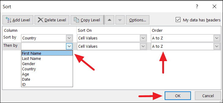
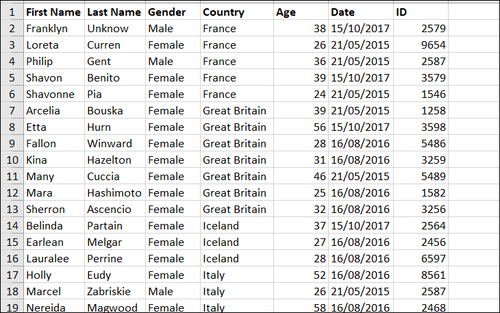
The data will now be sorted first by country and then by first name within each country group.
Sorting Rows Alphabetically in Excel
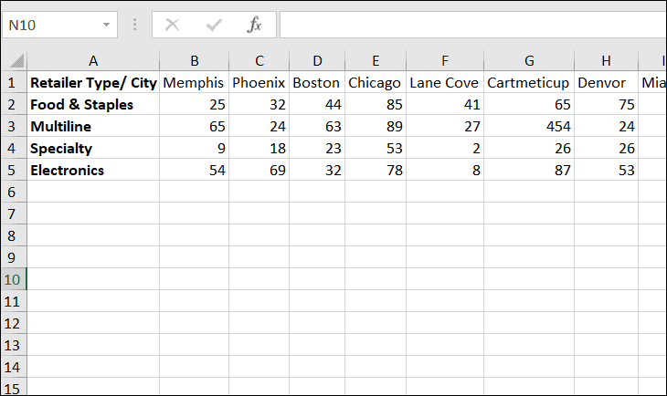
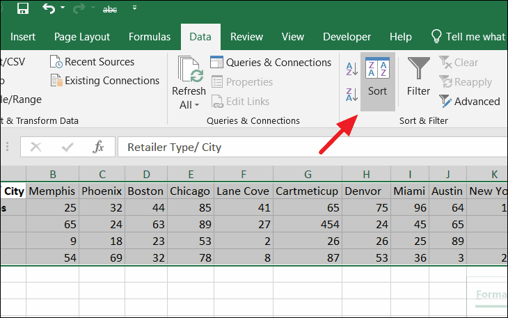
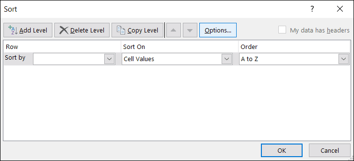
In some cases, you might need to sort data horizontally, alphabetizing rows instead of columns. Excel’s Sort feature can accomplish this by changing the sort orientation.
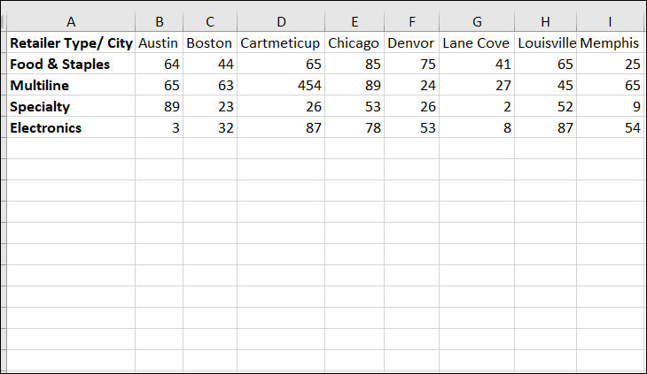
For instance, consider a spreadsheet where the first row contains city names across columns B to T, and column A lists retailer types. The sheet tracks the number of stores in each city for different retailer categories.
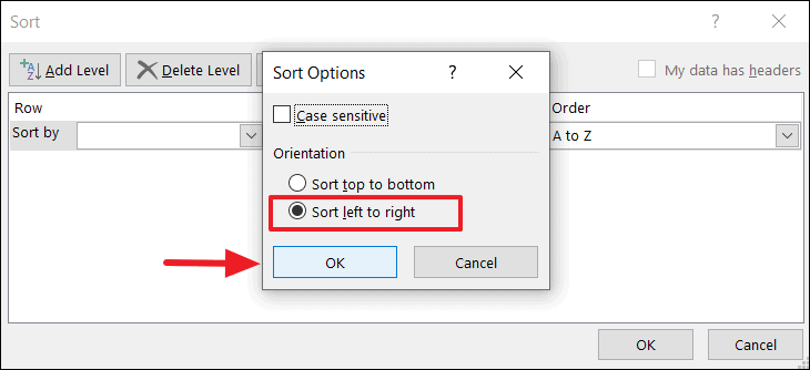
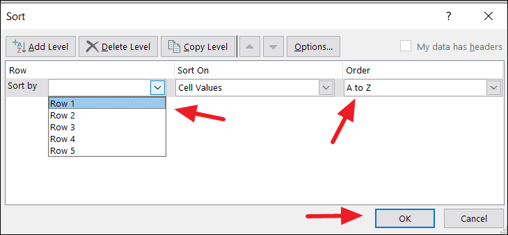
The first row will now be sorted in alphabetical order, and the data in the other rows will adjust accordingly.
Alphabetically Sorting a Column Using a Filter
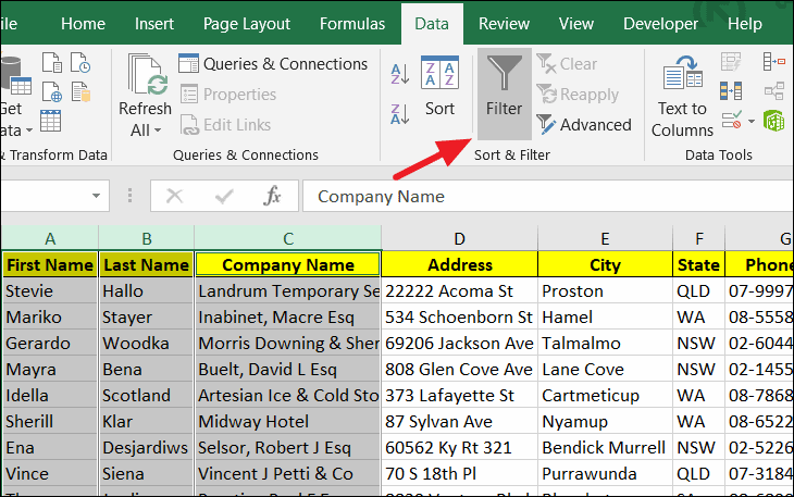
The Filter feature in Excel is another efficient way to sort data alphabetically. Applying filters to your columns provides quick access to sorting options.
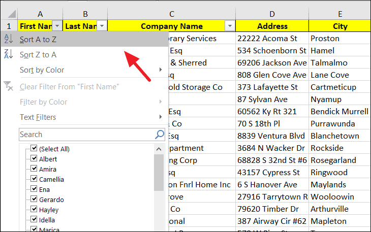
A drop-down arrow will appear in each column header.
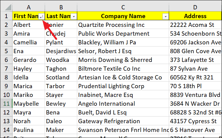
The column will be sorted in the chosen order, and a small arrow will indicate the sorting direction.
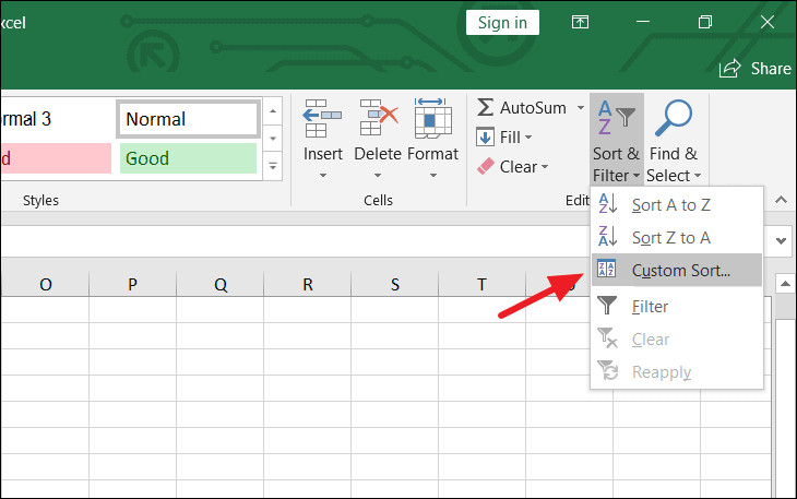
Advanced Sorting with Custom Order
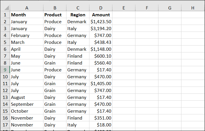
In certain cases, sorting data alphabetically might not be the most effective method. For example, lists containing months or weekdays are better sorted chronologically rather than alphabetically. Excel’s advanced custom sort options allow you to sort data based on custom lists.
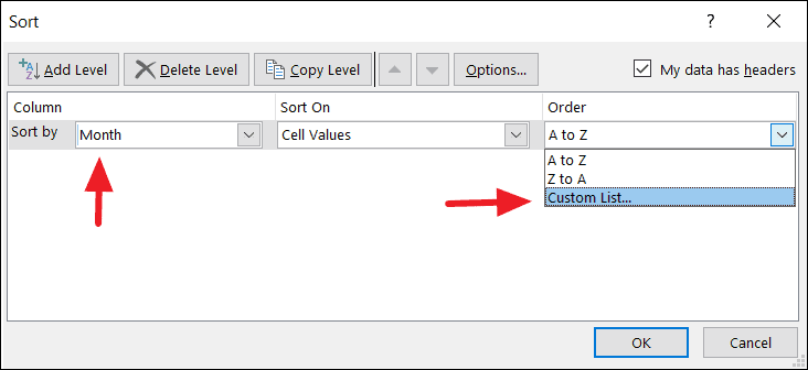
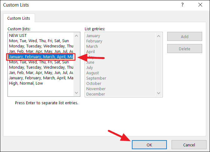
Your data will now be sorted based on the custom order specified, such as sorting months chronologically.
Alphabetizing Using Excel Formulas
Excel formulas can also be used to sort data alphabetically, which can be particularly useful for dynamic datasets that require automatic updating.
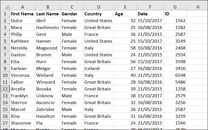
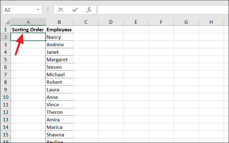
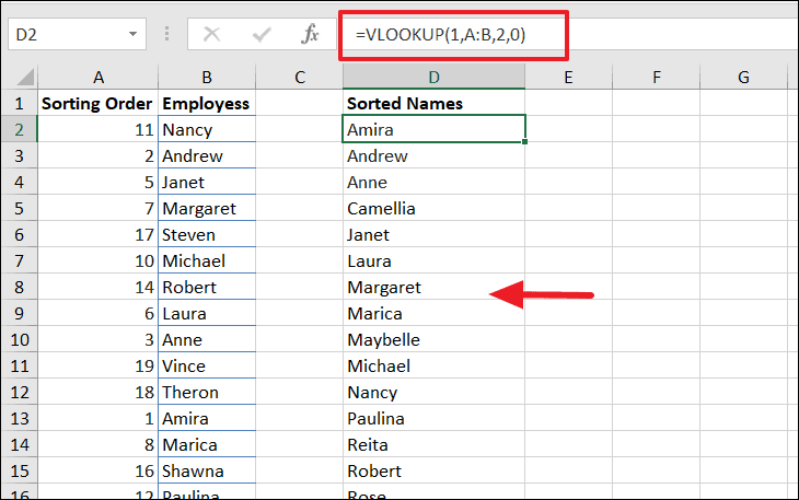
Suppose you have a list of names in column B that you want to alphabetize using formulas.
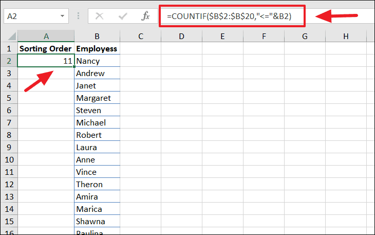
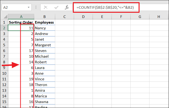
=COUNTIF($B$2:$B$20,"<="&B2)This formula counts how many names in the range B2:B20 are less than or equal to the name in B2, effectively determining its alphabetical position.
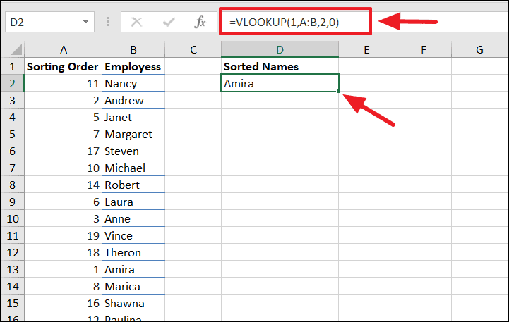
VLOOKUP function to retrieve the names in alphabetical order based on the sorting order numbers. In cell D2, enter:=VLOOKUP(ROW()-1,$A$2:$B$20,2,FALSE)This formula looks up the name that corresponds to the sorting order number.
Alphabetizing Entries by Last Name
Sometimes, you may need to sort a list of full names alphabetically by last name. This requires extracting the last names and using them for sorting.
=LEFT(A2,SEARCH(" ",A2)-1)=RIGHT(A2,LEN(A2)-SEARCH(" ",A2))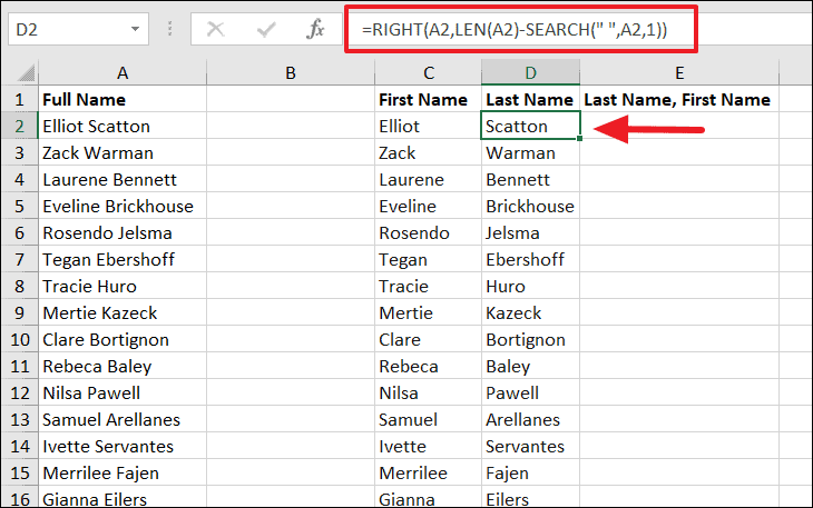
=D2&", "&C2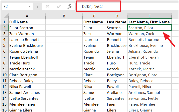
=RIGHT(E2,LEN(E2)-SEARCH(" ",E2))To extract the first name, and:
=LEFT(E2,SEARCH(" ",E2)-2)To extract the last name.
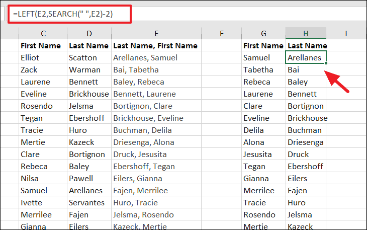
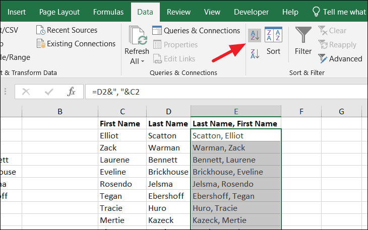
=FirstNameCell&" "&LastNameCellAfter these steps, you will have a list sorted by last name while maintaining the original name format.
Alphabetizing data in Excel enhances data management and accessibility. Whether sorting by a single column, multiple columns, or even rows, Excel provides robust tools to organize your data effectively.


