Formatting is a great way to make the contents of Excel cells more striking and stand out from the rest of the content. When you are working with large Excel sheets, you may apply various formatting to the cells such as changing cell color, font color, borders, alignment, number formatting, date formatting, conditional formatting, and others to customize your spreadsheet’s appearance.
Also, if someone shared a worksheet or you acquired your worksheet online, it’s more likely to be formatted. In such cases, you may like to apply different formatting or remove existing formatting from the sheet. However, deleting the contents of a cell doesn’t remove its formatting, so clearing up formatting could become a daunting task.
In this guide, we will show you several different ways to quickly remove formatting from specific cells of the worksheet or formatting applied to blank cells or the entire worksheet.
Clear Formatting for Select Cells in Excel
If you wish clear formatting from only a single or multiple select cells, you can do that without affecting any other cells in the worksheet. Here’s how you do that:
First, open the worksheet from which you want to remove the formatting. Now, highlight the cell or cells from which you want to remove all of the formattings.
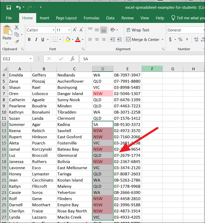
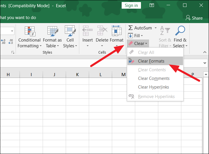
Next, go to the ‘Home’ tab, and click the ‘Clear’ (pink eraser icon) option in the Editing section at the right end of the Ribbon. Then, select the ‘Clear Formats’ option from the drop-down menu.
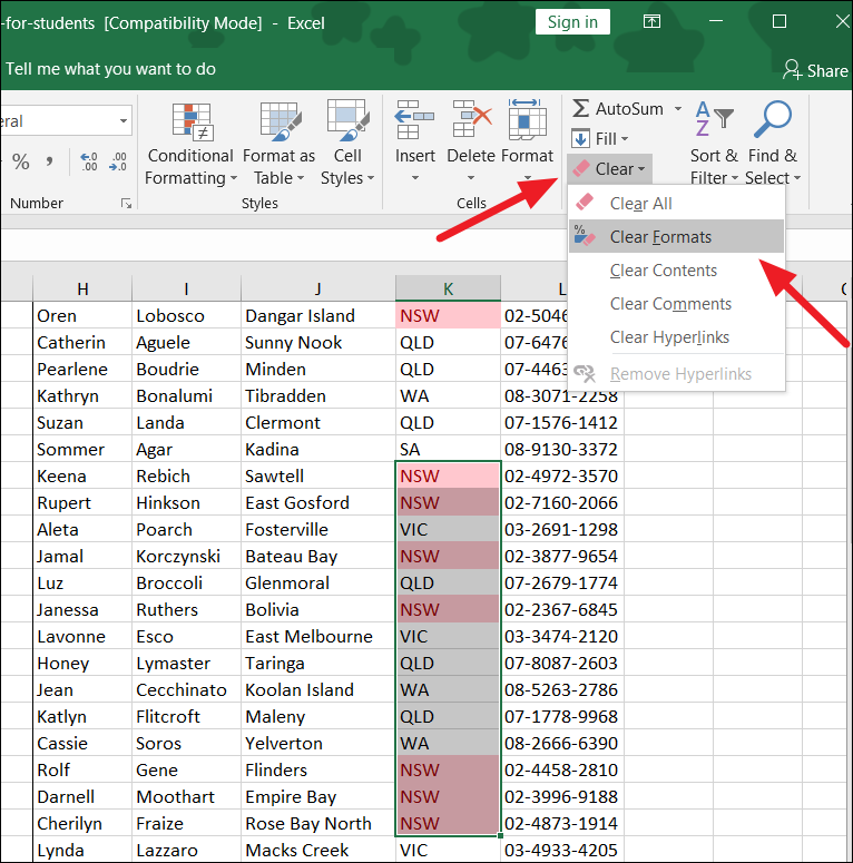
This will remove all the formatting of the selected cells leaving only the data behind.
Alternatively, you can also select the cells from which you want to remove the formatting and press this keyboard command: ALT+H+E+F.
Clear Formatting from the Entire worksheet in Excel
When you are working on a large spreadsheet with too many cells formatted, clearing them all separately would consume so much time. So, in that case, you can remove all the cell formatting from all the cells or the entire spreadsheet using the Clear feature.
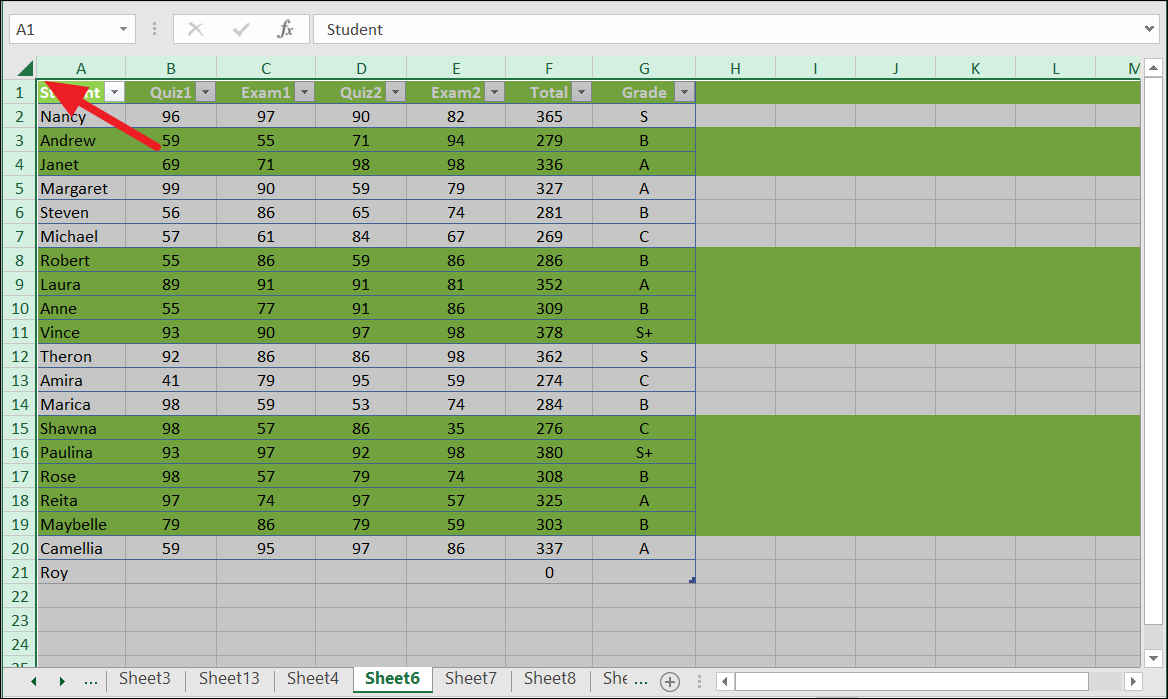
First, open your spreadsheet with the formatting. Now, click on the top left corner of the worksheet (one with a gray triangle icon) or press Ctrl+A to select all the cells in the worksheet.
Next, go to the ‘Home’ tab and click the ‘Clear’ option in the Editing group. Then, in the ‘Clear’ menu, click the ‘Clear Formats’ option.
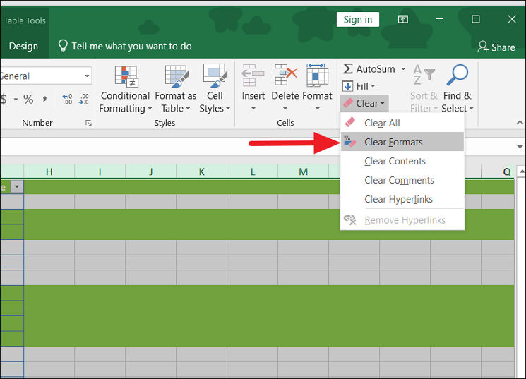
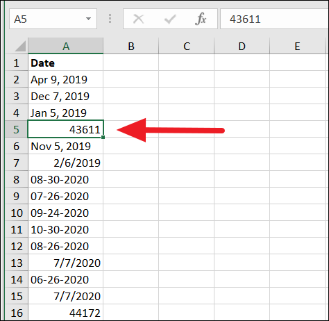
Remember removing formatting from the cell(s) will remove all types of formatting. For instance, if you remove formatting from cells that contain dates that are displayed in a certain date format (26-May-19), it will remove the date format and leave the serial number behind the date format: 43611.
Clear Only Contents from Cells while Keeping the Formatting of the Cells
You can also clear only the contents or data of the cells while keeping the formatting of the cells.
To do that, open the worksheet with formatted cells. Then, select the cells or the entire sheet from which you want to remove contents only.
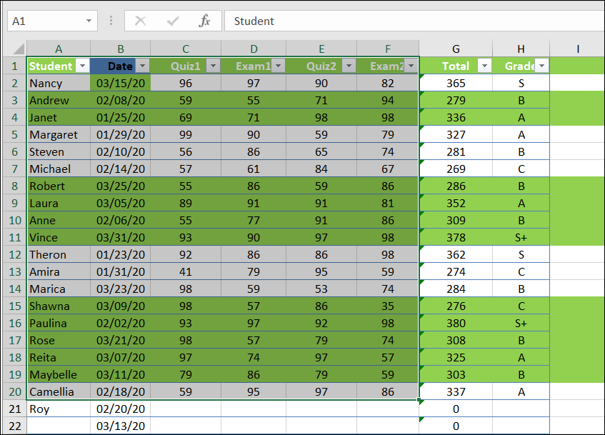
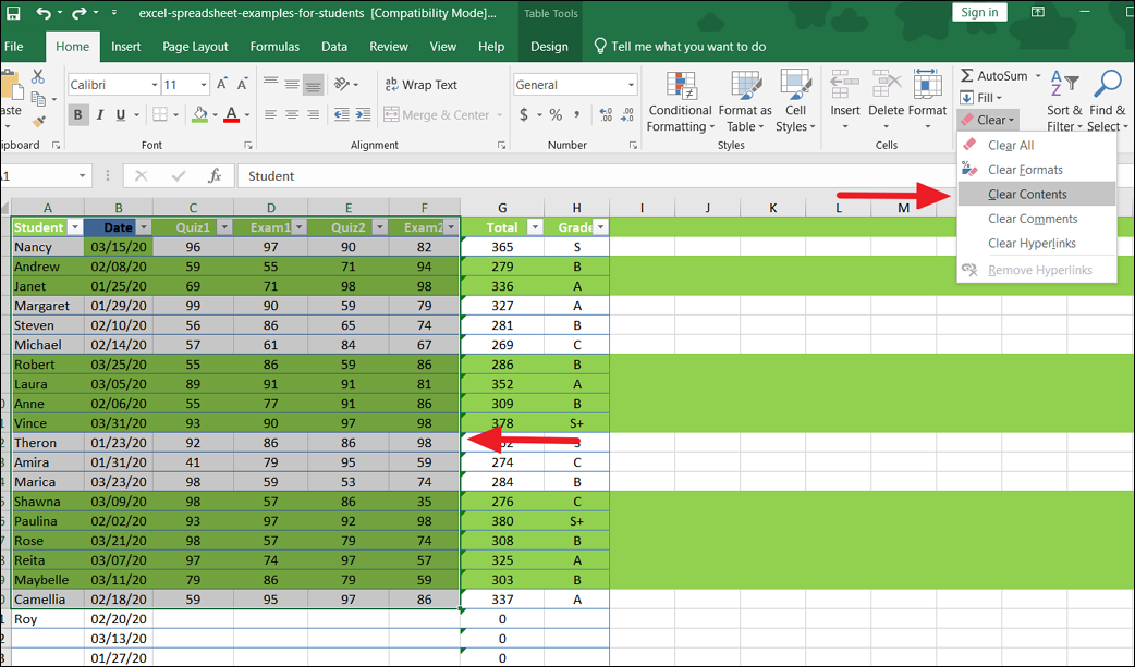
Then, go to the ‘Home’ tab, under the Editing section open up the ‘Clear’ menu (eraser button) and select ‘Clear Contents’.
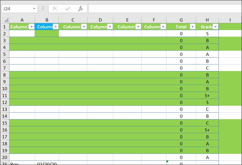
Now, all the cell data gets deleted from the selected range without any changes made to formatting.
Remove Formatting From Empty/Blank Cells
It is hard to notice if an empty cell has any formatting applied to it. So if you have a large spreadsheet with lots of empty cells, it will be challenging to find and remove formatting from all the empty or blank cells.
However, with Excel’s Go-To Special feature you can find the blank cells all at once and clear the formatting from them. Follow these steps to do this:
First, select the range of cells or the entire spreadsheet within which you want to select all the blank cells, then click the ‘Find & Select’ menu button from the Editing group of the ‘Home’ tab.
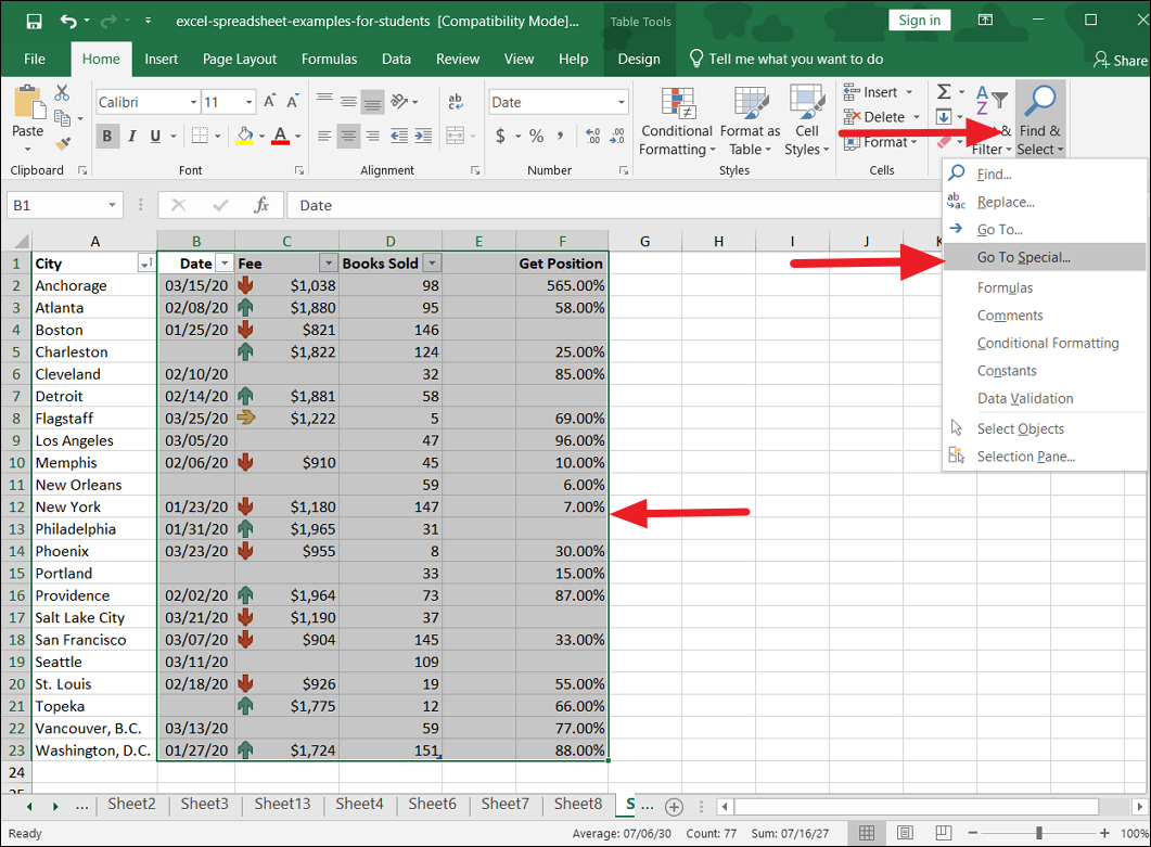
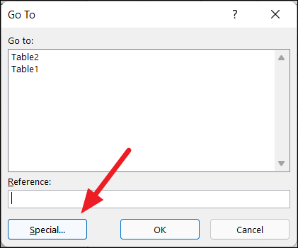
Alternatively, you can also select the range of cells with blank cells, press F5, and then click on the ‘Special’ button in the Go To dialog box.
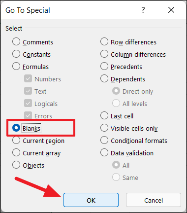
This will open the Go To Special dialog box. Here, select the ‘Blanks’ option and click ‘OK’.
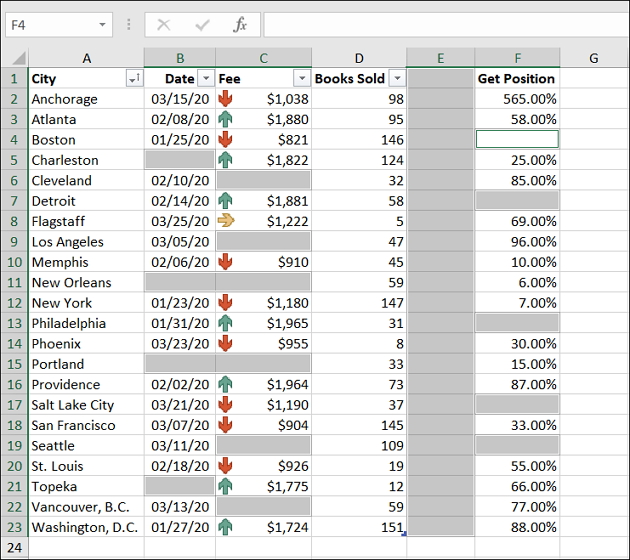
Doing this will select all the empty cells (highlighted in grey) in the selected range. Now, you can remove formatting from those cells.
To do that, go to the ‘Home’ tab and click the ‘Clear’ drop-down in the Editing group. Then, select the ‘Clear Formats’ option from the drop-down menu.
Using the same method, you can highlight all the blank cells and change the formatting as well.
Remove a Specific Cell Formatting from a Range/Worksheet
Occasionally, you may have a spreadsheet where you need to clear only a specific type of cell formatting from a range or a sheet. For instance, you may want to remove formatting from all the blue-colored cells or the cells that have negative numbers.
With the help of Excel’s Find and Replace feature, you can find and select cells that have specific formatting applied to them and remove them while keeping the rest.
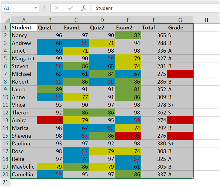
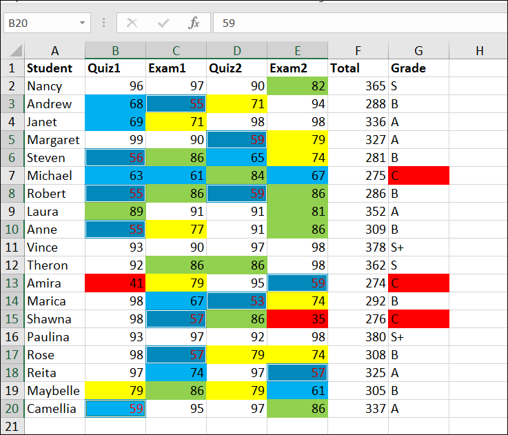
In the below dataset we have some cells that are formatted in blue cell color with red font color. We want to only remove that specific formatting while keeping the rest of the formatting in the sheet. To do that follow these instructions:
First, select the dataset with formatting or the entire worksheet.
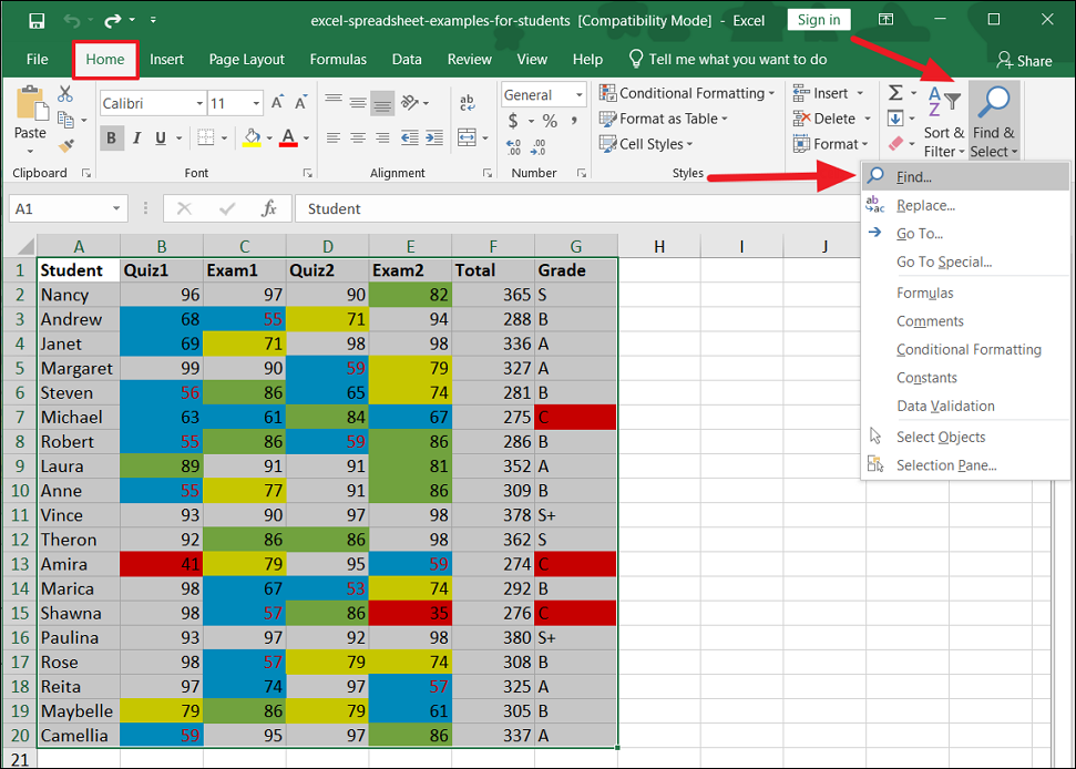
Then go to the ‘Home’ tab, click on ‘Find and Select’ in the Editing group and select ‘Find’.
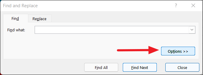
This will open the Find and Replace dialog box. Now, click the ‘Options’ button to expand advanced options.
Then, click on the drop-down icon (a downward pointing button) in the ‘Format’ button and choose the ‘Choose Format From Cell…’ drop-down menu.
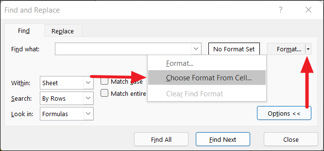
Doing this will change the cursor to a plus icon and a dropper. Now, simply select the cell that has the formatting you want to remove. Once you do that, you will see that the formatting you selected is shown in the ‘Preview’ box next to the ‘Find what:’ field (as shown below).
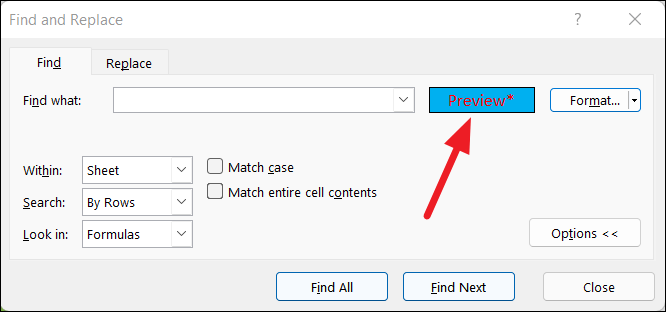
Confirm that is the formatting you want to remove and click the ‘Find All’ button.
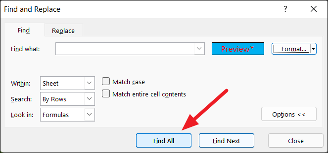
As soon as you do that, you will notice all the cell that has selected formatting will be listed below in the Find and Replace dialog box. Now, press the Ctrl+A shortcut to select all the listed results.
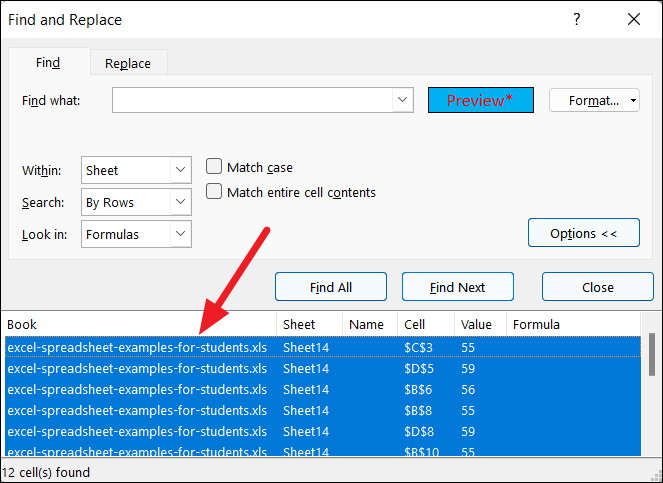
After that, click the ‘Close’ button to close the dialog.
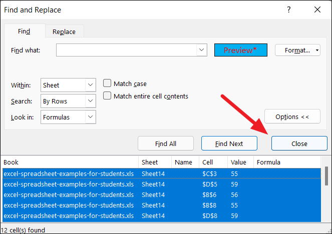
This will select all the cells with that specific formatting.
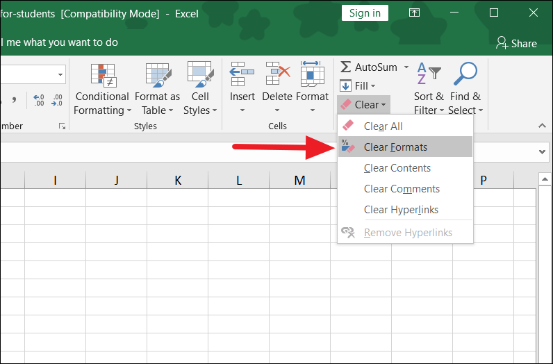
Now, click the ‘Clear’ button and select ‘Clear Formats’ in the Home tab.
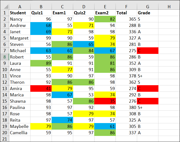
Once you do that, it will remove the specific formatting (blue cell color with red text) from the selected range.
Remove Current Formatting by Replacing Formatting from Another Cell
Another way to get rid of the formatting in a specific cell(s) is by copying a specific format (or no format) from another cell in your worksheet and pasting it in on the cell range. Here’s how you can do this:
First, copy the cell from which you want to copy the formatting by right-clicking and selecting ‘Copy’ or pressing Ctrl+C.
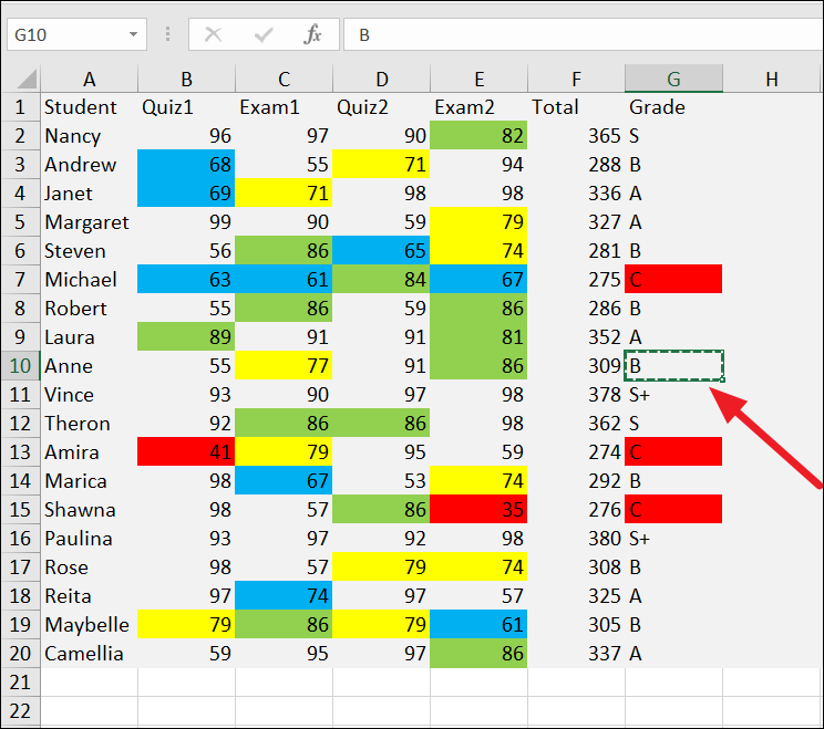
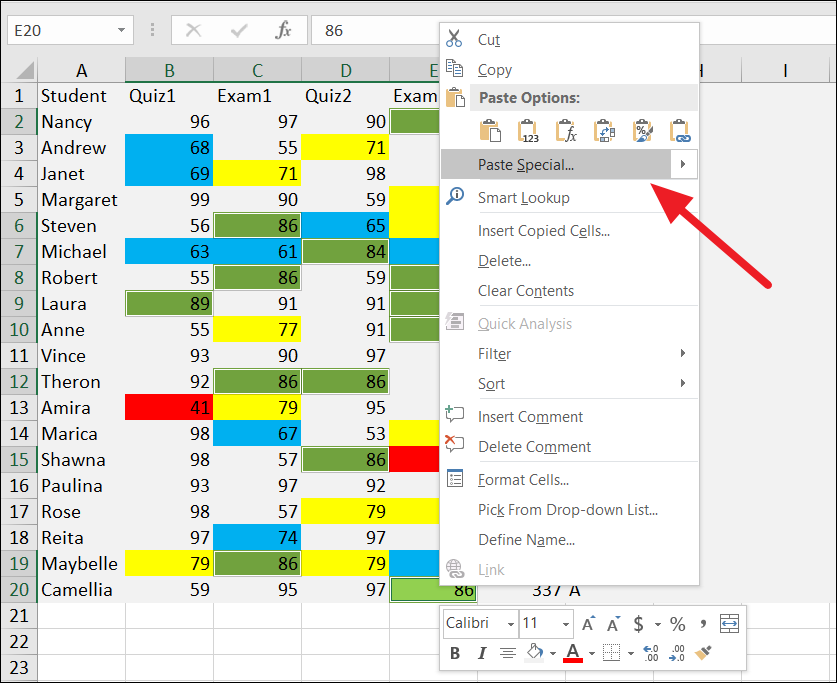
Next, select the cell(s) from which you want to remove the formatting and replace it with the copied formatting. Then, right-click on the selected cells and select ‘Paste Special…’
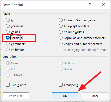
In the Paste Special dialog box, select the ‘Formats’ option under Paste and click ‘OK’.
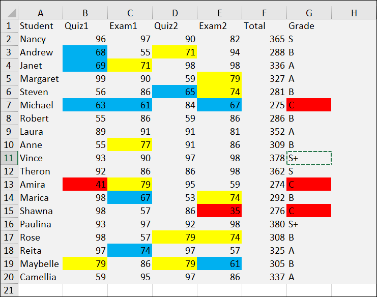
Doing this will apply the formatting from the copied cell to the selected cell(s) or range.
Clear Formatting using Format Painter
Format Painter is a tool in Excel that allows you to copy formatting from a cell(s) and apply it to a range of cells. You can also use Format Painter to remove formatting in Excel.
Select an empty cell with no formatting is applied. Then, go to the ‘Home’ tab and click on the ‘Format Painter’ (brush icon) button in the Clipboard group.
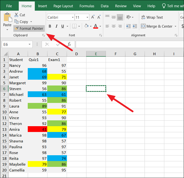
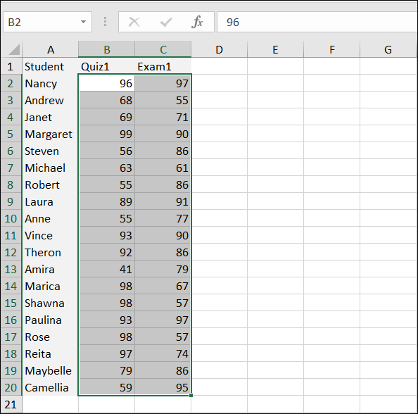
Now, just select all the cells from which you want to clear formatting. That’s it, all the formats will be cleared.
Clearing All Formats and Contents from Cells/Range/Worksheet
If you wish to remove everything including formatting, comments, contents, and hyperlinks from the cells, do this:
Select the cells or range for which you want to clear everything including formatting.
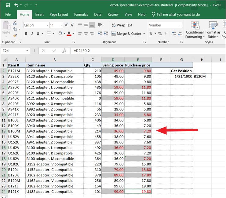
Go to the ‘Home’ tab, click the ‘Clear’ button under the Editing section, and select ‘Clear All’.
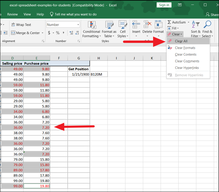
This will remove everything and turn the cells into blank cells.
Clear Formatting from Excel Table
When you convert a range of cells into a table, it is formatted with specific colors. If you try to remove formatting using the Clear Formats button, it won’t work. So if you want to remove table styles (format) from specific cells while keeping the rest of the table intact, follow these instructions:
For instance, if you remove cell color formatting in the below example using the Clear formats button, you will still see table style as shown below.
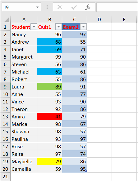
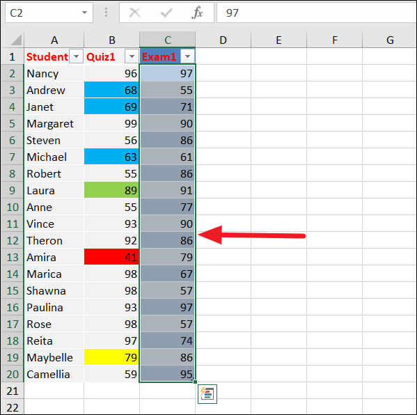
To remove table formatting from a range of cells, first, select the range from which you want to remove the formatting.
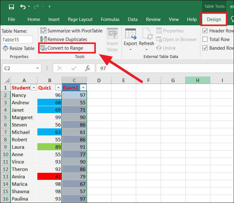
Next, go to the ‘Design’ or ‘Table Design’ tab and click the ‘Convert to Range’ button from the Tools group.
Then, click ‘Yes’ to the confirmation box.

Now, go back to the ‘Home’ tab and select the ‘Clear Formats’ button.
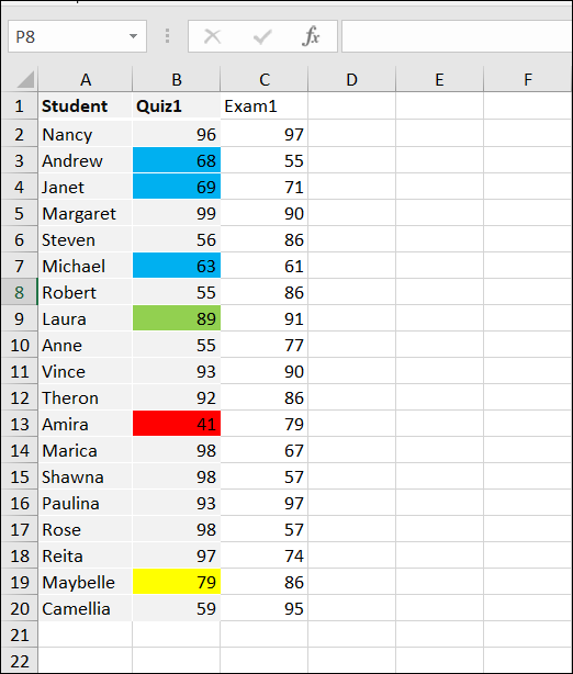
You can also remove the table formatting by clearing the Table Styles from the Design tab.
To do that, select the table or range of cells from which you want to remove the formatting.
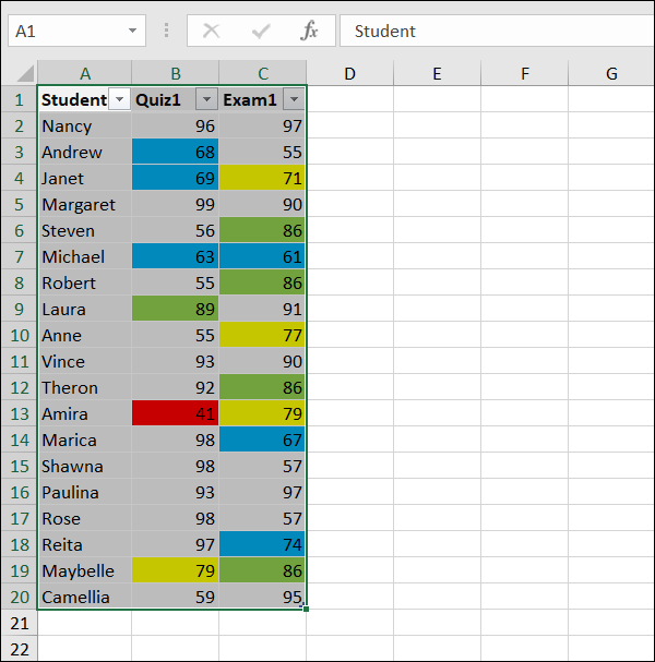
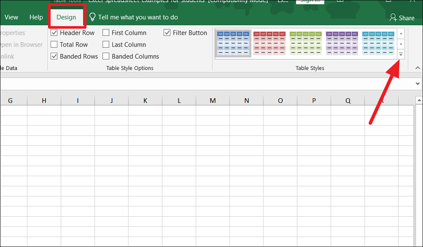
Next, switch to the ‘Design’ tab, and then from the ‘Table Styles’ group, select the ‘More’ button.
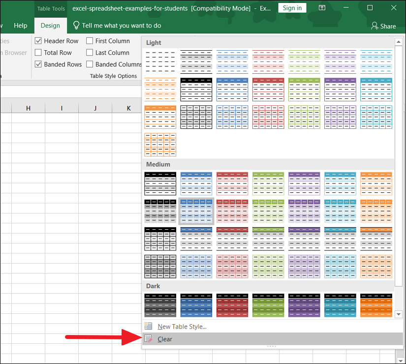
At the bottom of the expanded Table Style window, click the ‘Clear’ button.
Remove Conditional Formatting in Excel
In Excel, conditional formatting allows you to apply specific formatting to cells or ranges of cells based on a condition. If you want to remove conditional formatting in Excel, follow these steps:
To remove conditional formatting from a range of formatted cells, first, select the range. Then, go to the ‘Home’ tab, click the ‘Conditional Formatting’ option from the Style group, and click ‘Clear Rules’. Then, choose the ‘Clear Rules from Selected Cells’ option.
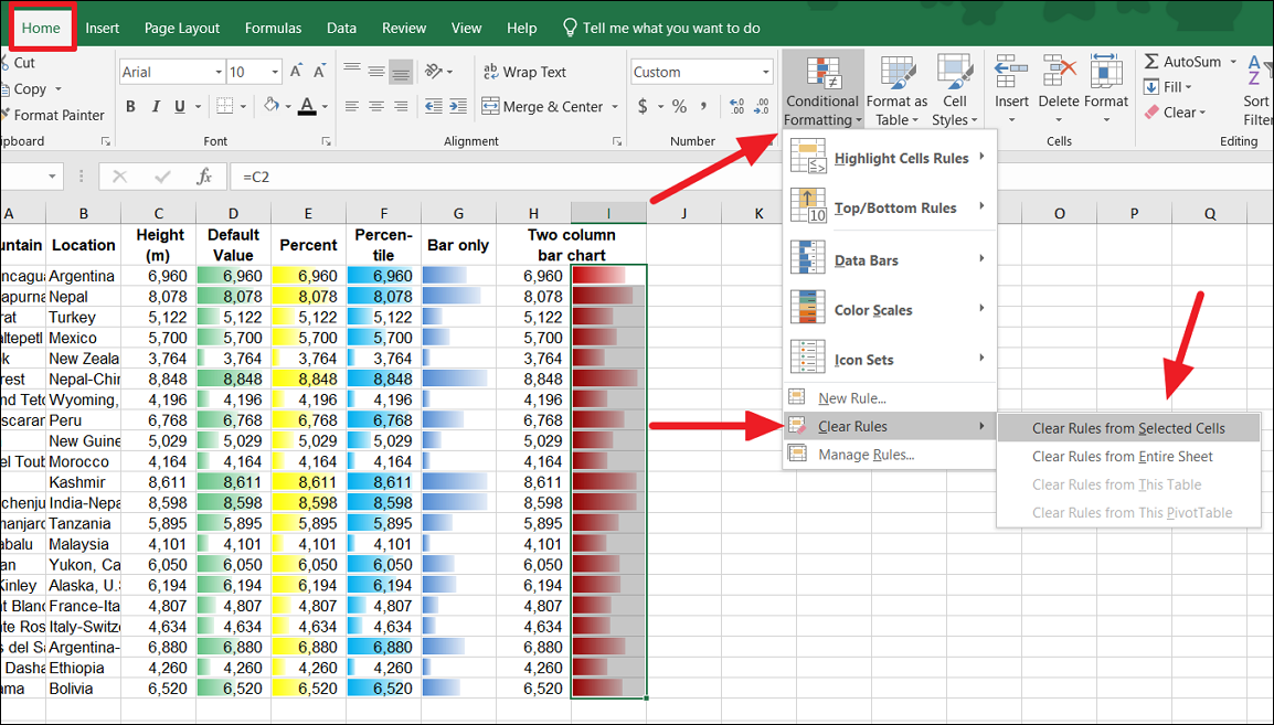
This will remove conditional formatting from only the selected range.
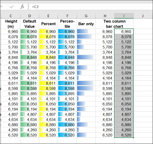
Alternatively, select any cell in the spreadsheet and from the ‘Home’ tab, click the ‘Conditional Formatting’ option in the Style group, and select ‘Manage Rules’.
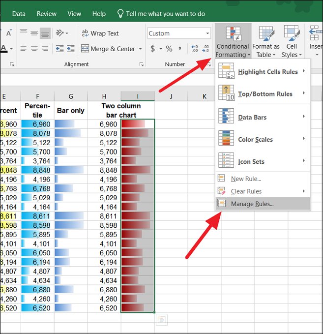
In the Conditional Formatting Rules Manager dialog box, select ‘This Worksheet’ from the ‘Show formatting rules for:’ drop-down.
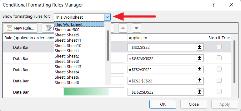
Then, select the rule (condition) you want to remove and click the ‘Delete Rule’ button.
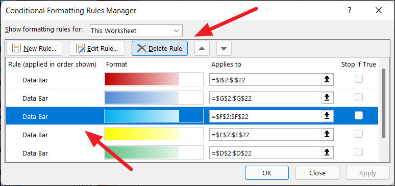
As a result, only that particular formatting rule is now cleared from the sheet.
To remove conditional formatting from the entire sheet at once, click the ‘Conditional Formatting’ option under the Home tab, and click ‘Clear Rules’. Then, choose the ‘Clear Rules from Entire Sheet’ option.
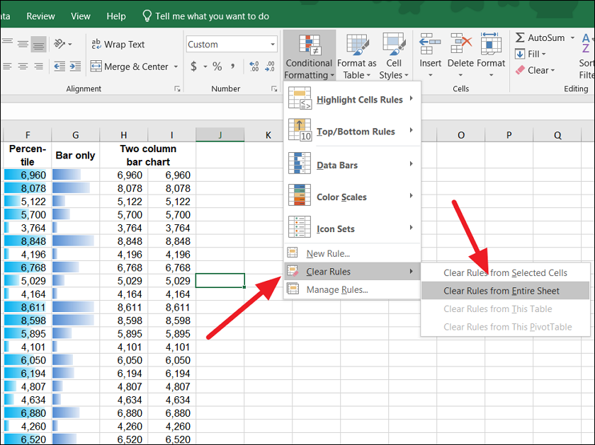
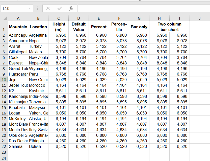
Now, all conditional formatting from the current worksheet is removed.
Adding the Clear Formats option to the Quick Access Toolbar
If you use the Clear formats tool frequently in your Excel, you can access it with one click by adding the tool to the Quick Access toolbar at the top of the ribbon. This is really helpful if you have lots of spreadsheets and you often need to remove formatting from them. To add the Clear Formats button to the Quick Access toolbar, follow these steps:
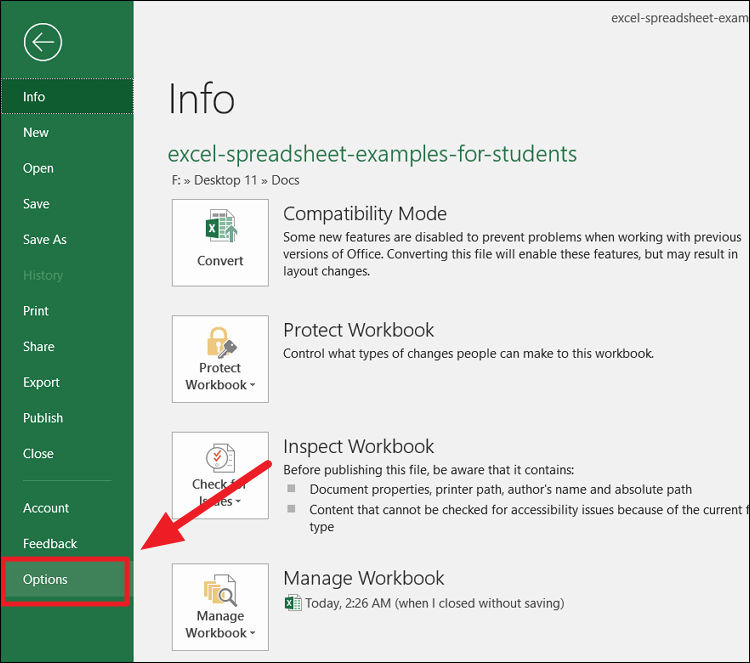
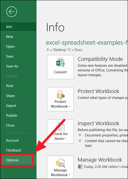
Open your Excel spreadsheet doesn’t matter which one, click the ‘File’ tab at the top left corner and select ‘Options’ from the backstage view left-sidebar.
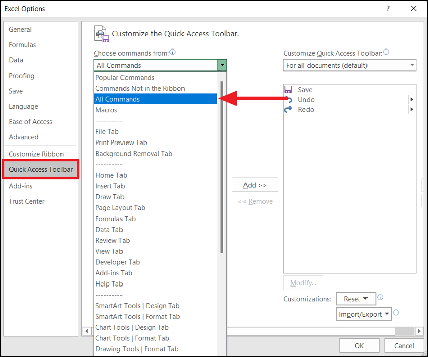
In the Excel Options window, click the ‘Quick Access Toolbar’ section in the left-side pane. From the ‘Choose commands from:’ drop-down, select ‘All Commands’ on the right-side pane.
Then, from the list of commands below, scroll down to the ‘Clear Formats’, select it, and then click the ‘Add’ button to move it to the right-hand box.
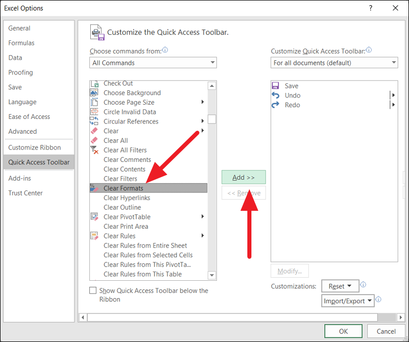
You can also add other commands such as Clear All, Clear Contents, Clear Hyperlinks, etc. to the right-side section. Once you are done, click ‘OK’.
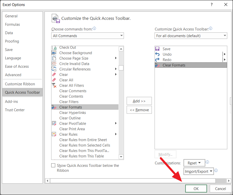
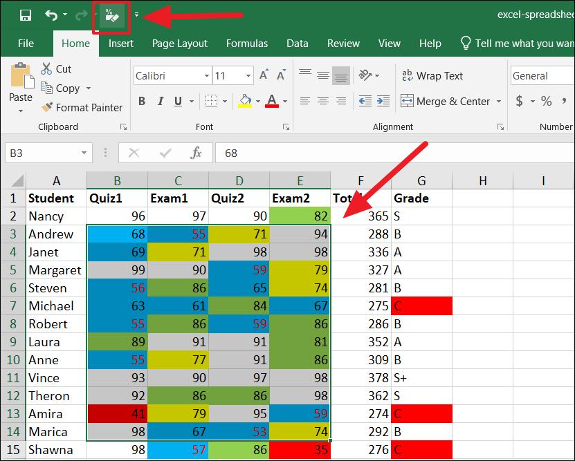
Now, the Clear Formats button is added to the Quick Access Toolbar at the top-left corner of the Excel window (where the undo, redo and save icons are located). All you have to do is select the range or the worksheet and click the ‘Clear Fromats’ on the Quick Access toolbar to remove formatting.
Add a Separate Clear Formats Button to the Ribbon
If you feel your Quick Access toolbar is filled with too many buttons, you can create a custom group on the Excel ribbon and add a separate ‘Clear Formats’ button in it which can be quickly accessed with a single click. Here’s how you add the ‘Clear Formats’ button to the Excel ribbon:
Open your Excel, click the ‘File’ tab at the top left corner and select ‘Options’ to open Excel Options.
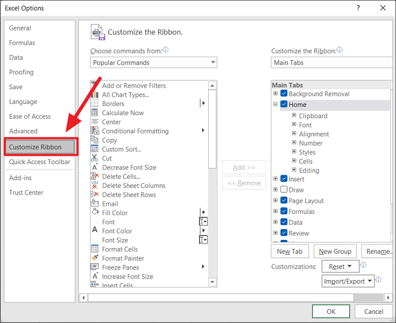
In the Excel Options window, click the ‘Customize the Ribbon’ section in the left-sidebar. Alternatively, you can right-click anywhere on the ribbon, and select ‘Customize the Ribbon’.
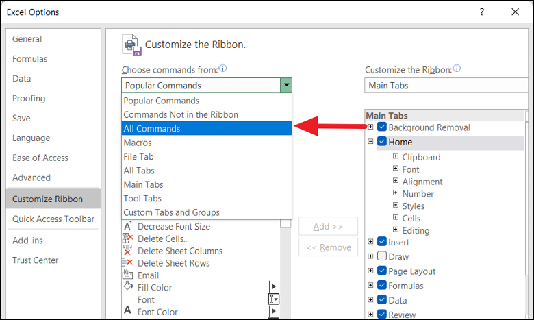
From the ‘Choose commands from:’ drop-down, select ‘All Commands’ on the right-side pane.
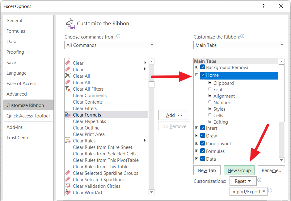
You can only add new commands to the custom groups in the ribbon. To do that, select the tab under which you want to add the custom group (In this case, Home) from the Main Tabs box, and click the ‘New Group’ button.
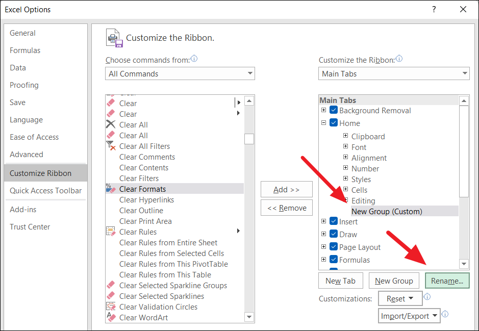
Now, select the ‘New Group (custom)’, and click the ‘Rename’ button below.
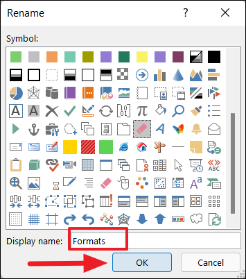
Then, enter a name for the group in the ‘Display name:’ field, choose Symbol if you want, and click ‘OK’.
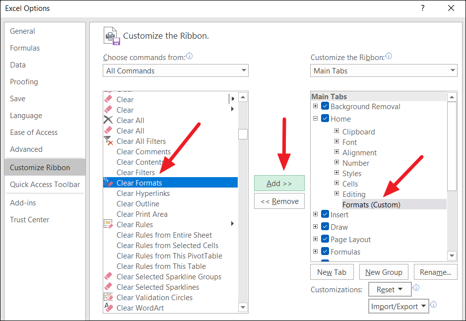
After that, select the newly created group (Formats (Custom)) under Main Tabs. Next, scroll down the list of commands under ‘Choose commands from:’ and select ‘Clear Formats’. Then, click the ‘Add’ button.
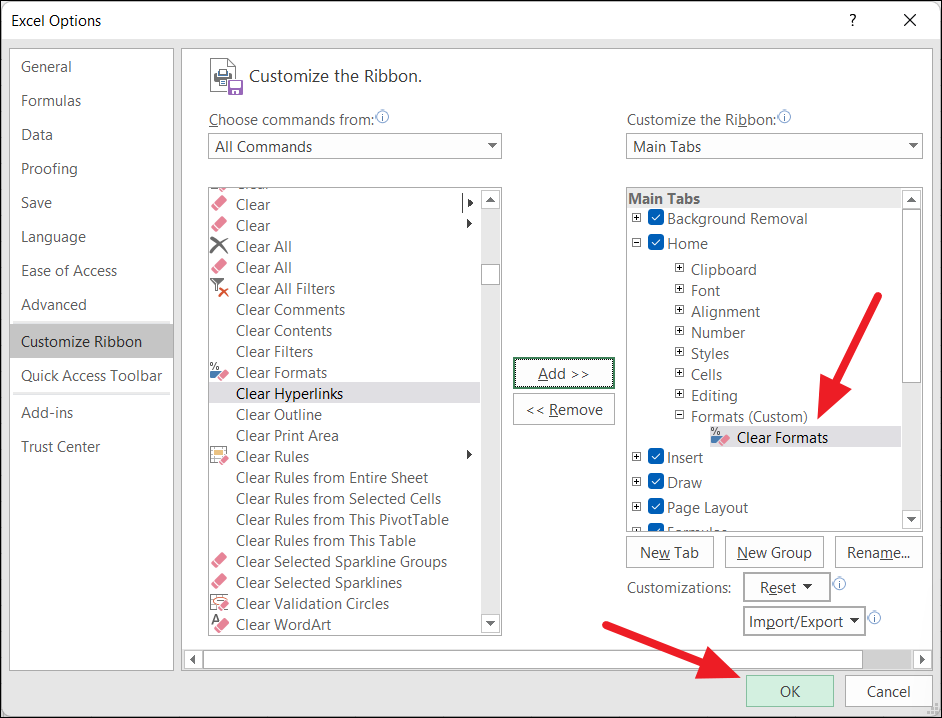
Then, click ‘OK’ to apply the changes.
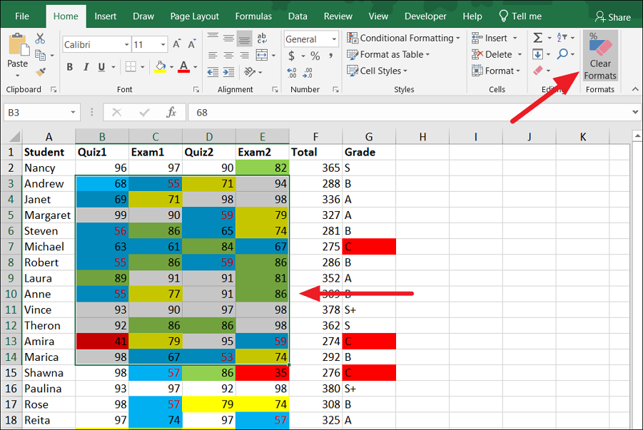
This will add a new button (Clear Formats) on the Ribbon, you can now clear formatting with a single click.
That’s it.

