
Efficiently duplicating formulas in Excel saves time and reduces the risk of errors like #REF! and #DIV/0! that can occur from incorrect cell references. Instead of retyping the same formula repeatedly, Excel provides several methods to copy formulas across cells, ranges, or entire columns.
Copying a Formula to an Entire Column or Row
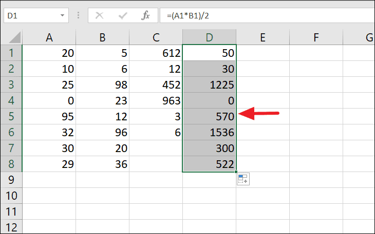
One of the quickest ways to replicate a formula across a column or row is by using the Fill Handle. This method allows you to extend a formula to adjacent cells without manually copying and pasting.
+).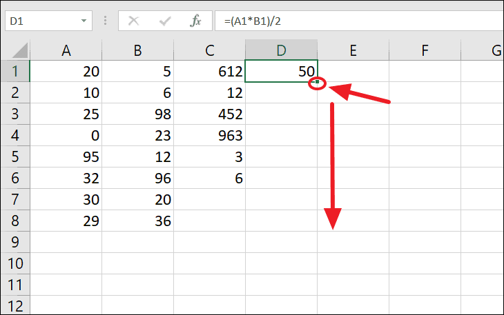
As you drag the formula, Excel automatically adjusts the relative cell references, ensuring that each cell calculates based on its corresponding row or column.
Tip: Double-clicking the Fill Handle will automatically fill the formula down the column as far as there is data in the adjacent column, saving you even more time.
Copying a Formula from One Cell to Another
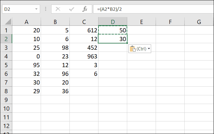
Sometimes you may need to copy a formula to a single, non-adjacent cell. Instead of retyping the formula, you can copy and paste it efficiently.
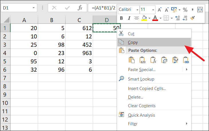
Ctrl + V to paste it. Alternatively, you can right-click the destination cell and select ‘Paste’ or ‘Formulas’ under the ‘Paste Options’.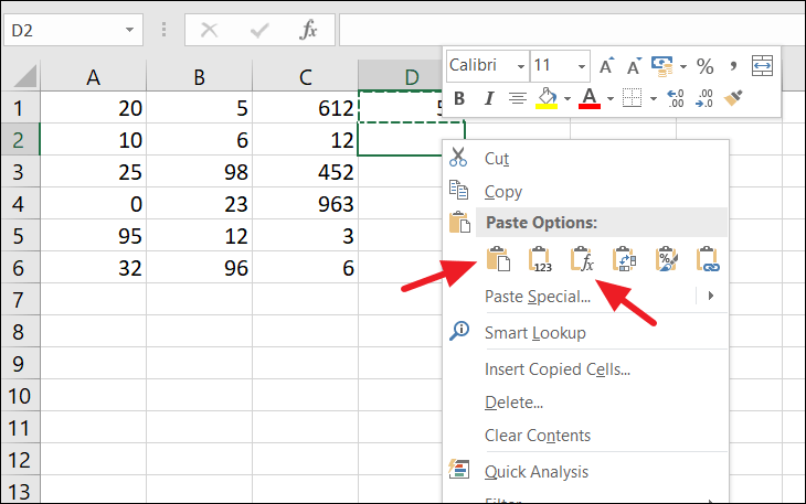
The pasted formula will adjust its cell references relative to the new location, ensuring accurate calculations.
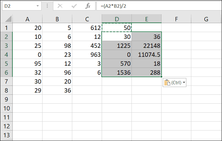
Copying a Formula from One Cell to Multiple Cells
To apply a formula to multiple non-adjacent cells or a specific range, you can use the copy and paste method.
Copying a Formula to Non-Adjacent Cells
Applying a formula to cells that are not next to each other is straightforward with Excel’s copy and paste features.
Ctrl key, click on each non-adjacent cell where you want to paste the formula.Ctrl + V to paste the formula into all of them simultaneously.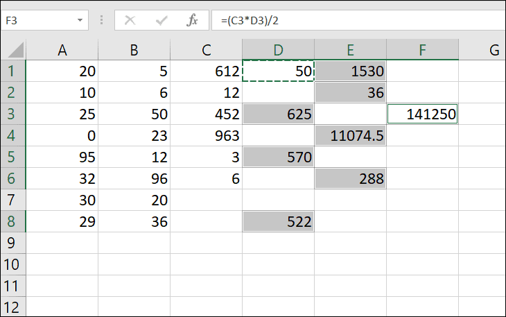
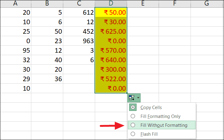
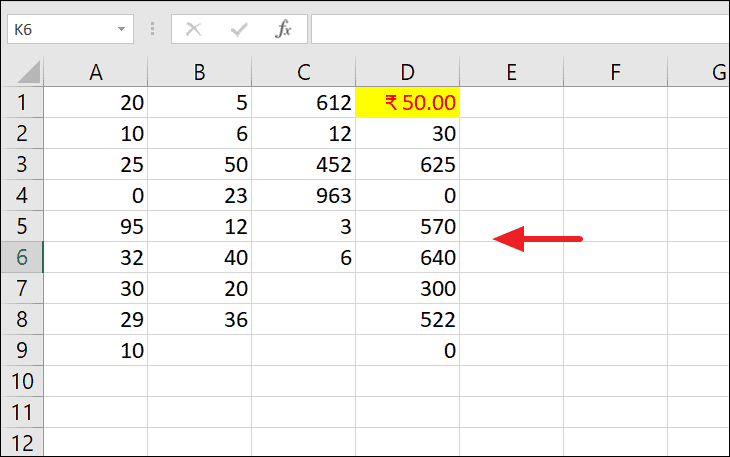
Copying a Formula Without Formatting
When copying formulas, Excel also copies the cell’s formatting by default, which might not always be desired. To copy only the formula without any formatting, follow these steps.
Copying Formulas Without Changing Cell References
By default, when you copy formulas, Excel adjusts the cell references relative to their new positions. To copy a formula exactly as it is, without changing the cell references, you can employ absolute references or use specific copy methods.
Using Absolute Cell References
To prevent cell references from changing, convert them to absolute references by adding dollar signs ($) before the column letter and row number.
Copying Formulas Exactly Using Copy-Paste Method
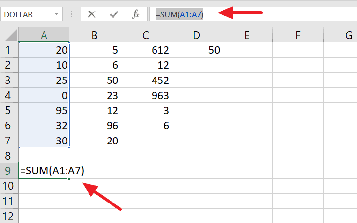
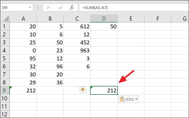
This method copies the formula exactly, without altering any cell references.
Using Find and Replace
You can use the Find and Replace feature to temporarily modify formulas for copying.
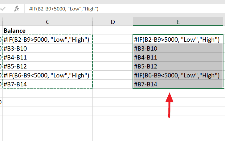
=. In the ‘Replace with’ field, enter a unique character or string, such as #=, and click ‘Replace All’. This converts your formulas to text strings.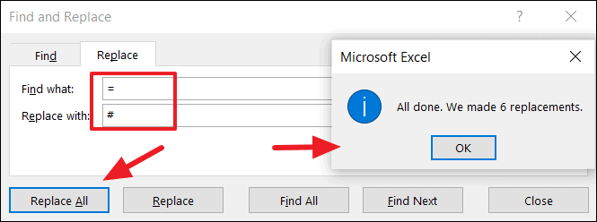
Ctrl + H), replace the unique character or string (e.g., #=) with =, and click ‘Replace All’ to restore the formulas.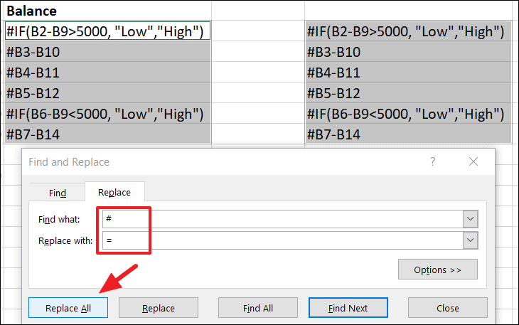
Now, the formulas are copied exactly without any changes to the cell references.
Copying Formulas and Preserving Number Formatting Only
If you need to copy a formula along with specific number formatting (such as decimal places, currency symbols, or percentage formats) but without other cell formatting, you can use the ‘Formulas & Number Formatting’ paste option.
% fx).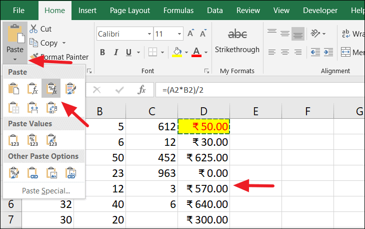
This method applies the formula and preserves the number formatting while ignoring other cell formats like font color or cell fill color.
By utilizing these methods, you can efficiently copy and paste formulas in Excel, ensuring accurate calculations and saving time in your spreadsheet tasks.


