How to Display Cell Formulas in Excel

By default, when you type a formula in a cell and hit enter, Excel shows the result of the formula and hides the formula underneath it. However, when working with huge amounts of data and lots of formulas, sometimes you may need to show the formulas in the cells instead of the outputs for several reasons.

Those reasons include displaying formulas for printing, editing the formula, understanding the dependencies, correcting errors and mistakes, etc. Displaying cell formulas can help you keep track of data (or the cells containing the data) used in each formula and verify the entered formulas for any possible errors.

Whatever reason you have, we will show you several different methods for displaying the cell formulas in Excel.

Show the Cell Formula using the Formula Bar

The formula bar is the easiest and fastest way to view or edit the entered formula in Excel. The downside is that you can only view one formula at a time.

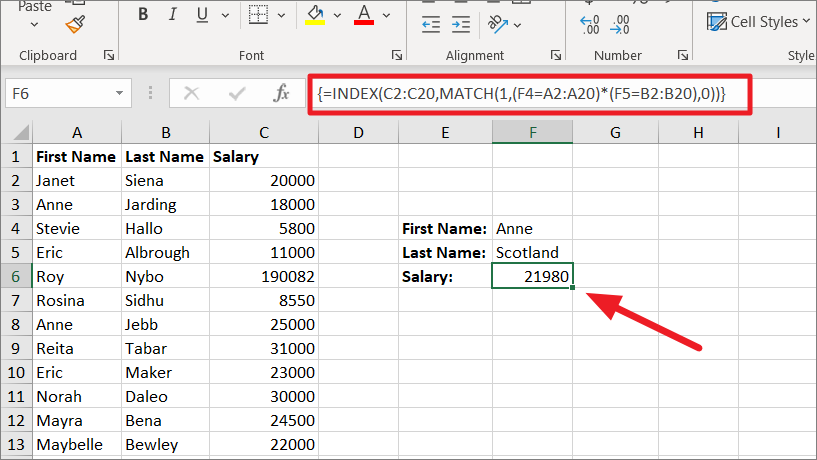
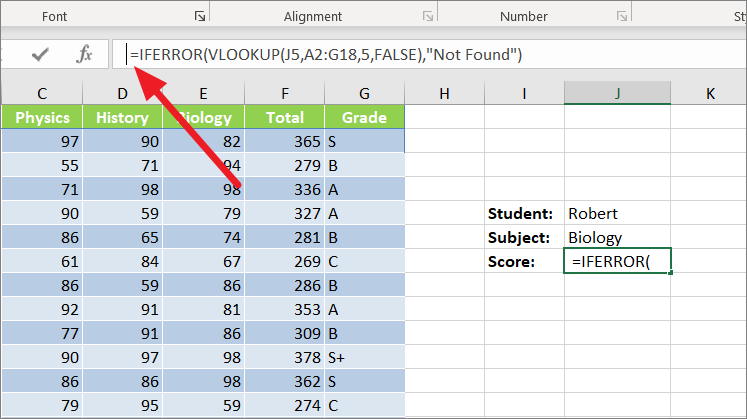
First, open the spreadsheet in which you want to view the formula. If you know which cell contains the formula, simply select that cell and you will see the formula in the Formula Bar right below the Ribbon.

Show Formula using Double-Click

If you want to view a single formula within a cell itself instead of the Formula bar, then just double click on that cell.

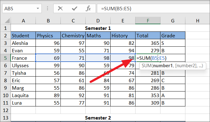
Simply, double-click on the cell with the formula, and Excel will reveal the formula in Edit mode as shown below.

Display Excel Formulas using Keyboard Shortcut

Another quickest way to display cell formulas is using keyboard shortcuts which show all the formulas entered in a spreadsheet.

Simply press Ctrl+` (Grave Accent Key). You can find the Grave Accent Key right above the Tab key on the left side of your keyboard.

Now, if you want to show results instead of the formulas, press the Ctrl+` again.

Display the Formulas using the Show Formulas command

Another method you can use to show formulas in all cells in the current worksheet is using the Show formulas command from the ribbon. Here’s how:

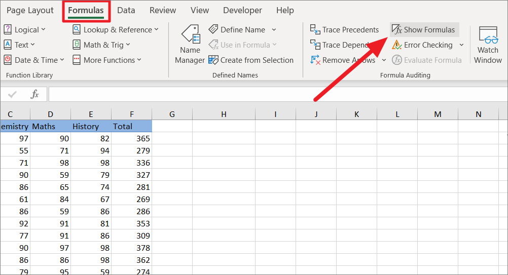
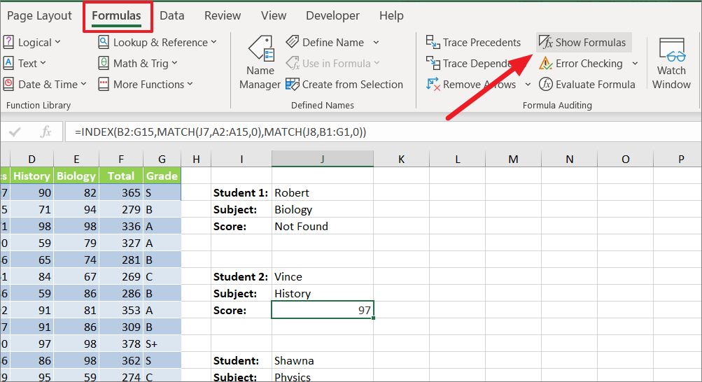
Open the spreadsheet in which you want to show all the formulas. Then, go to the ‘Formulas’ tab and click the ‘Show Formulas’ option in the Formula Auditing group.

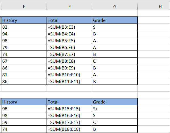
Excel will now show all the formulas in the worksheet.

To show values again in the cells, go back to the ‘Formulas’ tab and toggle the ‘Show Formulas’ command again.

Show Formulas in Cells Instead of Their Results

This method required a few more steps than the previous methods, but with this method, Excel can show formulas in several worksheets instead of their results. Follow these steps to display formulas in cells instead of their results:

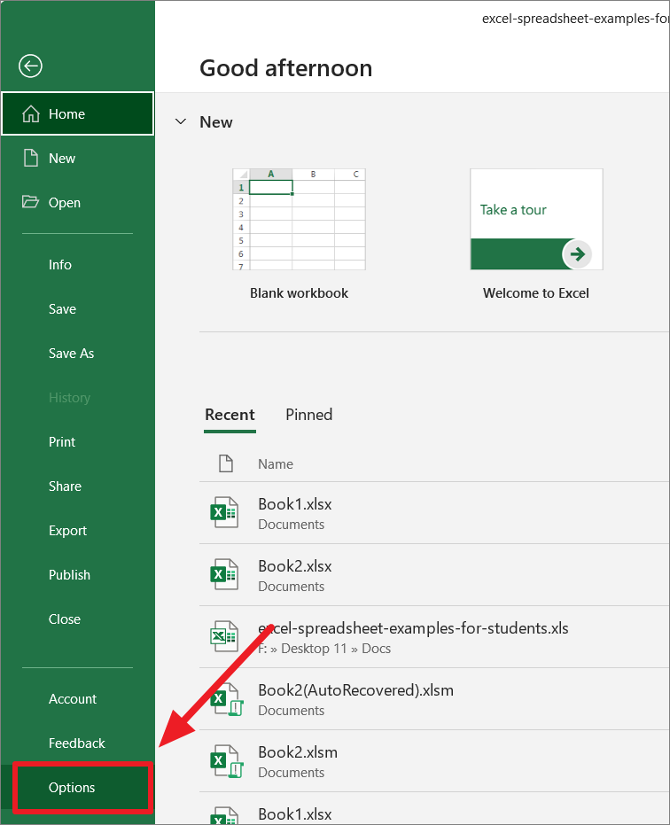
First, go to the ‘File’ tab and select ‘Option’ from the backstage view.

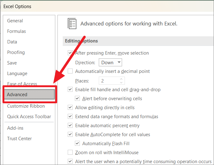
In the Excel Options window, select ‘Advanced’ from the left-side panel.

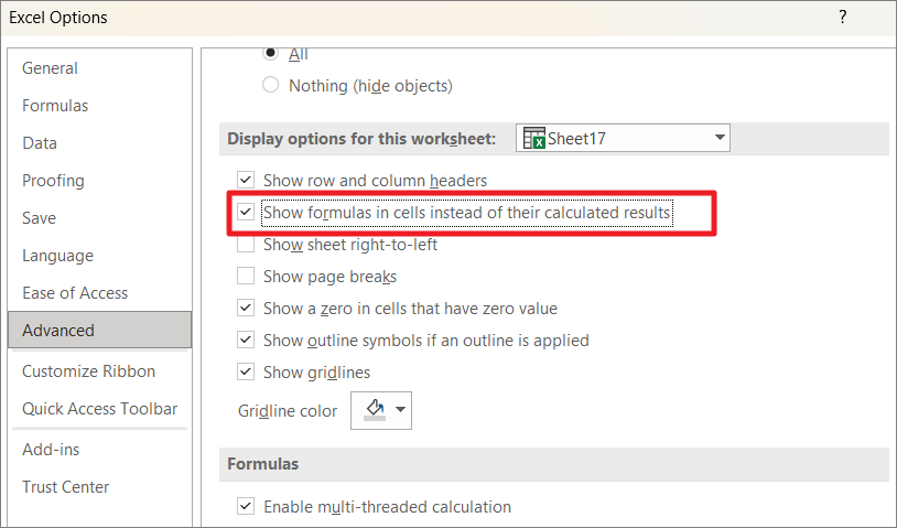
On the right side, scroll down to the ‘Display options for this worksheet’ section. Then, from the drop-down list, select the sheet in which you want to display the formulas. You can select any sheet from the current workbook as well as sheets from any other open workbook.

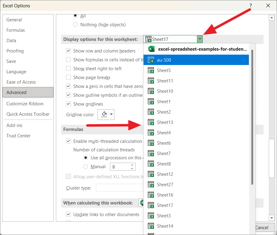
Now, check the ‘Show Formulas in cells instead of their calculated results’ option.

When you enable the ‘Show Formulas in cells..’ option in a specific sheet all other worksheets will be unaffected. To display formulas in other sheets, you will need to select that sheet from the drop-down and enable this option.

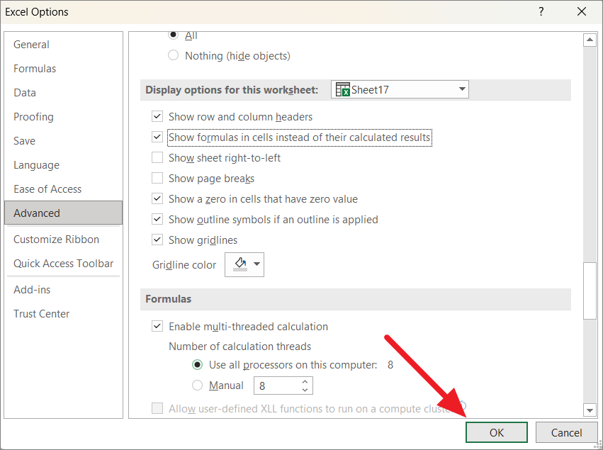
After that, click ‘OK’ to apply the changes.

Now, all formulas will be displayed in the specific sheet. If you want to show results instead of the formula again, go back to the Advanced options and uncheck the box ‘Show formulas in cells instead of calculated results’ option.

Use the FORMULATEXT Function to Display Formulas in Cell

If you prefer to use formulas, you can use the FORMULATEXT function to show the formula from a specific cell in another cell as a text string. You can use this method if you want to show both formulas and result at the same time in two separate cells.

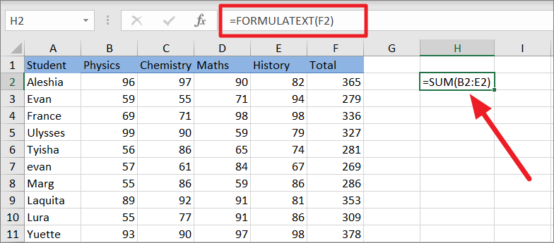
First, select the cell where you want to display the formula and type the below formula:

=FORMULATEXT(F2)

Where F2 refers to the cell that contains the formula. If you refer to a cell that does not contain a formula, it will return a #N/A error. As you can see, the formula is displayed in cell H2 and the value in F2.

Display Formulas in Selected Cells Only

All the above methods can help you show formulas in either a single cell or all the cells in the worksheet but not only in specific cells of the sheet. If you want to display formulas in only selected cells in the sheet, you can use the find and replace trick to do it:

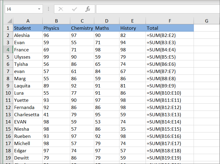
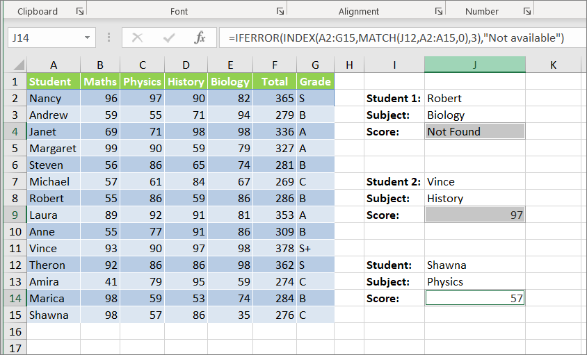
Let’s assume we have the below spreadsheet:

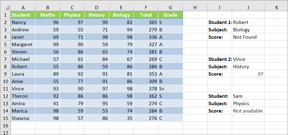
In the above sample data, if we use Ctrl+` shortcut or ‘Show Formulas’ option from the ribbon, Excel will reveal all the formulas in the sheet.

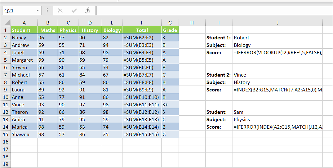
But we don’t want that, we only want to display the formulas in cells J4, J9, and J14, but not the formulas in column F. To do that, follow these steps:

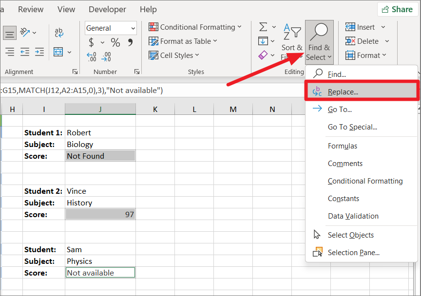
First, select all the cells where you want to display the formula instead of the value.

Go to the ‘Home’ tab, click ‘Find & Select’ and select the ‘Replace’ option from the drop-down. Or press Ctrl+H.

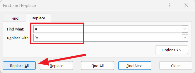
In the Find and Replace dialog box, under the Replace tab, type = in the ‘Find what’ field and ‘= in the ‘Replace with’ field. Then, click the ‘Replace All’ button.

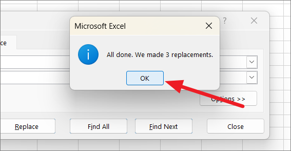
After that, click ‘OK’ and then ‘Close’ to exit both dialog boxes.

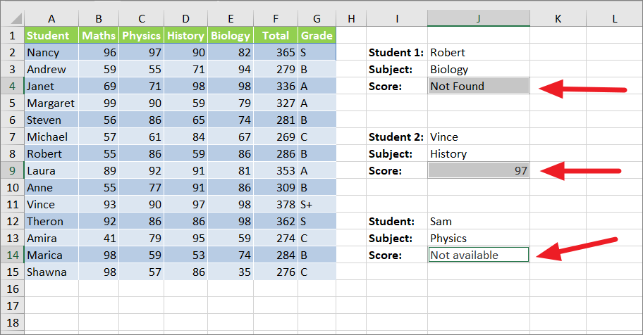
Now only the formulas in the selected cells will be displayed while the other cells (with formulas) would not be changed as shown below.

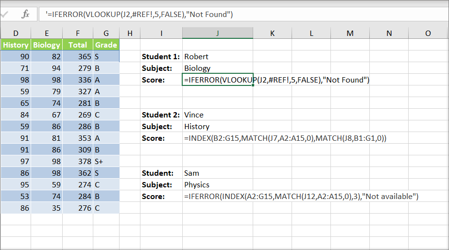
By adding the apostrophe (‘) symbol before the ‘equal to’ sign, we are making the formula a text string and displaying it in the cell.

Also, the apostrophe (‘) symbol we added before the = sign in the formula will be hidden in the cells and it would only show up in the formula bar when you select the cells.

Format the Cell as Text to Display Formula

Another method to display formulas in cells is to set the cell format to Text. However, you need to set the cell’s formatting to Text before entering the formula for this to work.

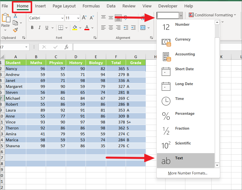
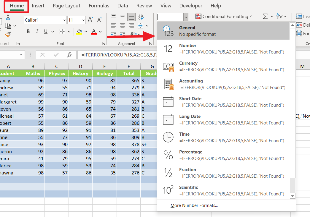
Select the cell where you want to enter the formula and display it. Then, go to the ‘Home’ tab, click the drop-down from the Numbers group and select ‘Text’.

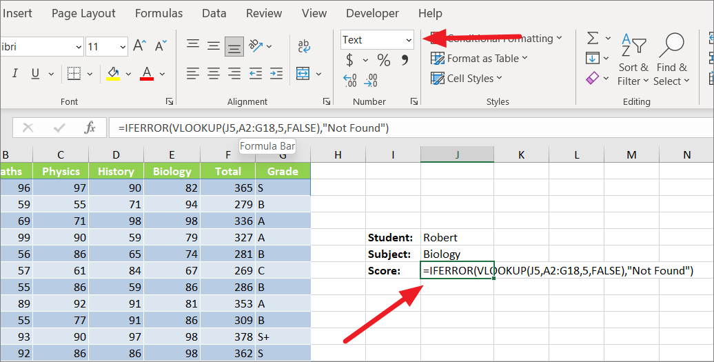
After setting the cell formatting text, you can enter the formula in the cell and it will remain visible as a text string.

If you want to show the result instead of the formula, change the cell formatting to ‘General’, click on the Formula bar and then press Enter.

Hide Formulas Completely in Excel

Sometimes, you don’t want to show formulas but instead, hide them completely from prying eyes. If you are sharing a spreadsheet that contains some complicated formulas and you don’t want other users accidentally changing the formulas and messing up your calculations, you can hide them and protect the sheet. This method will prevent the formulas in the cells from being viewed or edited. Here is how it’s done:

First, select the cells whose formulas you want to hide. You can also select only specific cells in the sheet or the entire worksheet. In the below example, we want to hide formulas in cells J4, J9, and J14.

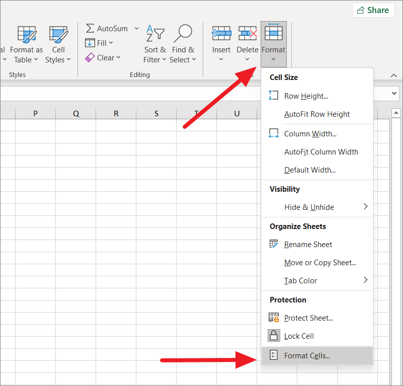
Next, go to the ‘Home’ tab, and click ‘Format’ in the Cells group on the right side of the ribbon. Then, select the ‘Format Cells’ option from the drop-down menu.

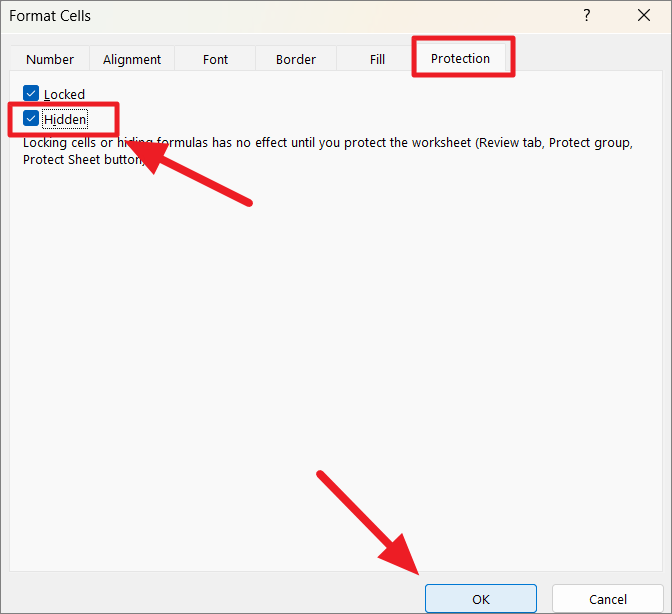
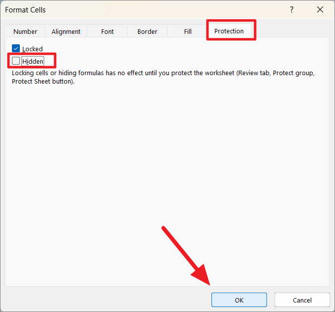
When the Format Cells dialog box opens up, switch to the ‘Protection’ tab, and check or select the ‘Hidden’ option. Then, click ‘OK’.

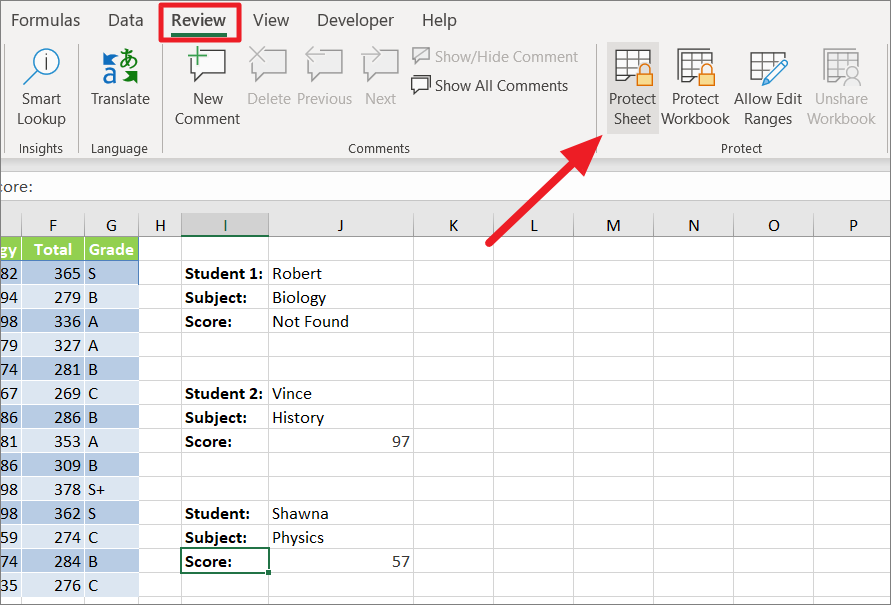
After that, you need to protect the worksheet to fully hide the formulas in the Excel sheet.

To do that, head to the ‘Review’ tab and click the ‘Protect Sheet’ option in the Protect section.

This will open a small Protect sheet dialog box. Here, enter a password in the ‘Password to unprotect sheet’ edit box and make sure the ‘Protect worksheet and contents of locked cells’ option is selected.

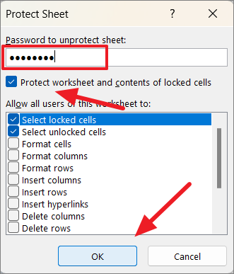
Under the ‘Allow all users of this worksheet to’ box, select the functions that you want to allow the users to execute. Then, click ‘OK’.

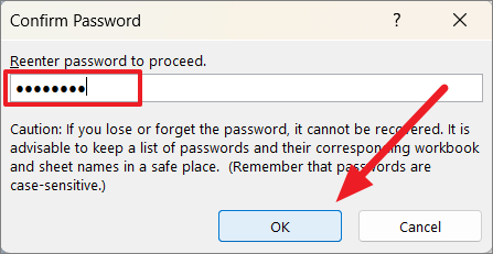
You will be asked to confirm the password. Re-enter the password in the field and click ‘OK’.

Once you do that, all the locked and hidden cells will be password protected.

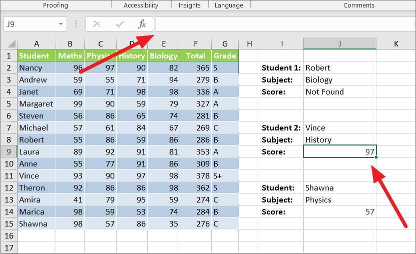
Now, if you select a cell with a formula, the formula bar will be blank as shown below.

If you wish to display the formulas again, you will need to unprotect the worksheet with the same password.

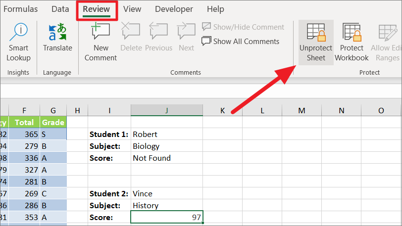
To unprotect a spreadsheet, go back to the ‘Review’ tab and select the ‘Unprotect Sheet’ option in the Protect section.

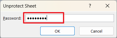
Now, enter the password (you used to protect the sheet with) on the Unprotect Sheet dialog box and click ‘OK’.

Next, go back to the ‘Home’ tab, click ‘Format’ and select ‘Format Cells’. Under the ‘Protection’ tab, uncheck the ‘Hidden’ option, and click ‘OK’.

Now, the worksheet will be unprotected and the formulas will be unhidden.

How to Fix Excel Showing Formulas Instead of Values issue?

Every now and then, you may find that your Excel worksheet shows formulas instead of their calculated results even when you haven’t used any of the above methods to display formulas. There are multiple reasons for this, let us see some of the potential solutions that might fix this issue.

Disable ‘Show Formulas’ option or Press Ctrl+`

You may have accidentally enabled the ‘Show Formulas’ command from the ribbon or pressed Ctrl+` shortcut. To show values again, simply hit the Ctrl+` shortcut again or toggle the ‘Show Formulas’ option from the Formula tab.

Remove Unnecessary Characters before the Formula

If Excel thinks your formula is text, it will display the formula as text instead of calculating the formula. It could be due to a space character, apostrophe, or any other character before the equal sign in the formula. If the formula is wrapped in double-quotes or the absence of an equal sign before the formula will also turn the formula into a text.

In such cases, make sure to remove the leading space, apostrophe, or other characters before the formula.

Change the Cell Formatting

If you set the cell formatting to Text and you enter the formula in that cell, Excel will consider that formula as text and does not calculate it.

To solve this problem, select the formula cell, go to the ‘Home’ tab, click the drop-down in the Number group, and change the formatting to ‘General’.