
While working in Google Sheets with large data sets, you probably run into a problem where you have to deal with many duplicate values. While some duplicates entries are placed intentionally while others are mistakes. This is especially true when you are collaborating on the same sheet with a team.
When it comes to analyzing data on Google Sheets, being able to filter out duplicates can be essential and convenient. Although Google Sheets doesn’t have any native support for finding duplicates in sheets, it offers several ways to compare, identify, and remove duplicate data in cells.
Sometimes, you want to compare each value in a column with another column and find if there are any duplicates in it and vise versa. In Google Sheets, you can easily find duplicates between two columns with the help of the conditional formatting feature. In this article, we will show you how to compare two columns in Google Sheets and find duplicates between them.
Find Duplicate Entries Between Two Columns using Conditional Formatting
Conditional formatting is a feature in Google Sheets that allows the user to apply specific formattings such as font color, icons, and data bars to a cell or range of cells based on certain conditions.
You can use this conditional formatting to highlight the duplicates entries between two columns, either by filling the cells with color or changing the text color. You need to compare each value in a column against another column and find whether any value is repeated. For this to work, you have to apply conditional formatting to each column separately. Follow these steps to do that:
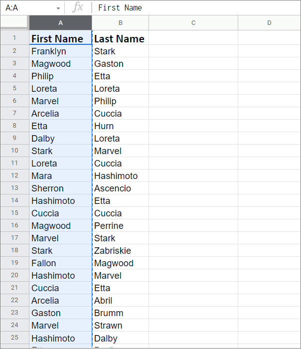
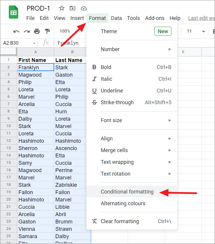
Open the spreadsheet you want to check for duplicates in Google Sheets. First, select the first column (A) to check with column B. You can highlight the entire column by clicking on the column letter above it.
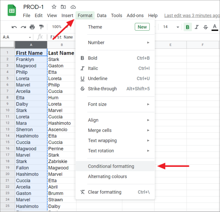
Then, click the ‘Format’ menu from the menu bar and select ‘Conditional formatting’.
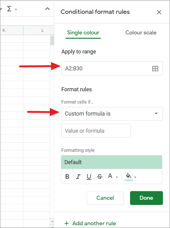
The Conditional Formatting menu opens on the right side of the google sheets. You can confirm the cell range is what you selected under the ‘Apply to range’ option. If you want to change the range, click the ‘range icon’ and choose a different range.
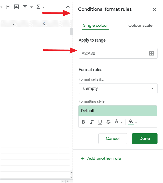
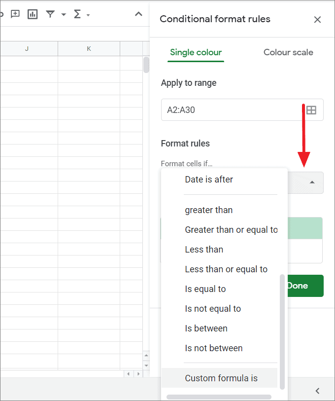
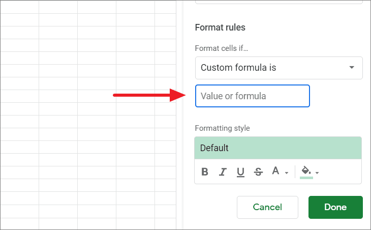
Then, click the drop-down under ‘Format rules’ and select the ‘Custom formula is’ option.
Now, you need to enter a custom formula in the ‘Value or formula’ box.
If you selected an entire column (B:B), enter the following COUNTIF formula into the ‘Value or formula’ box under Format rules:
=countif($B:$B,$A2)>0Or,
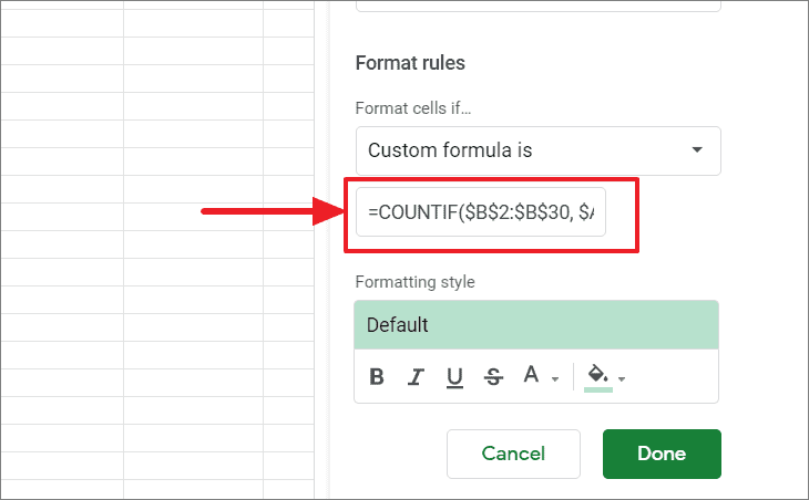
If you selected a range of cells in a column (say a hundred cells, A2:A30), use this formula:
=COUNTIF($B$2:$B$30, $A2)>0When you are entering the formula, make sure to replace all instances of the letter ‘B’ in the formula with the letter of the column you’ve highlighted. We’re adding the ‘$’ sign before the cell references to make them absolute range, so it doesn’t change we apply the formula.
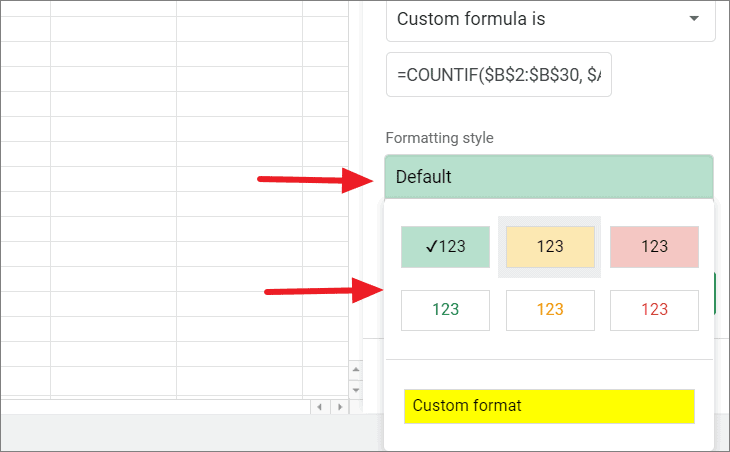
In the Formatting style section, you can choose the formatting style for highlighting the duplicate items. By default, it will use the green fill color.
You can choose one of the preset formatting styles by clicking on the ‘Default’ under the ‘Formatting style’ options, then selecting one of the presets.
Or, you can use any of the seven formatting tools (Bold, Italic, Underline, Strikethrough, Text colour, Fill colour) under the ‘Formatting style’ section to highlight the duplicates.
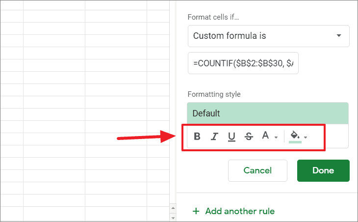
Here, we choosing a fill color for the duplicate cells by clicking the ‘Fill colour’ icon and selecting the ‘yellow’ colour.
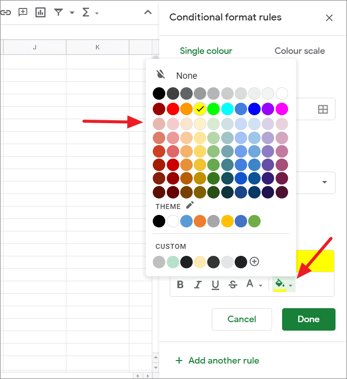
Once you selected the formatting, click ‘Done’ to highlight the cells.
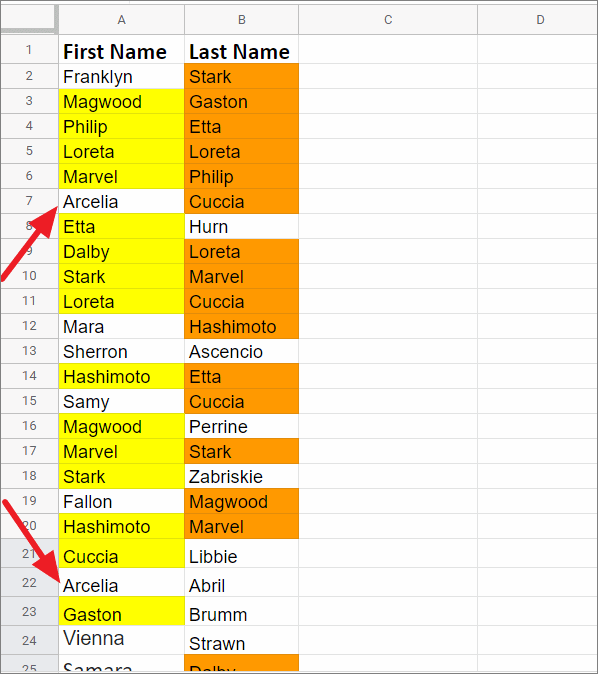
The COUNTIF function counts how many times each cell value in ‘Column A’ appears in ‘Column B’. So if an item appears even once in column B, the formula returns TRUE. Then that item will be highlighted in ‘Column A’ based on the formatting you chose.
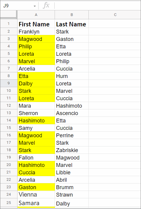
This doesn’t highlight the duplicates, but rather it highlights the items that have duplicates in Column B. That means each yellow highlighted item has duplicates in Column B.
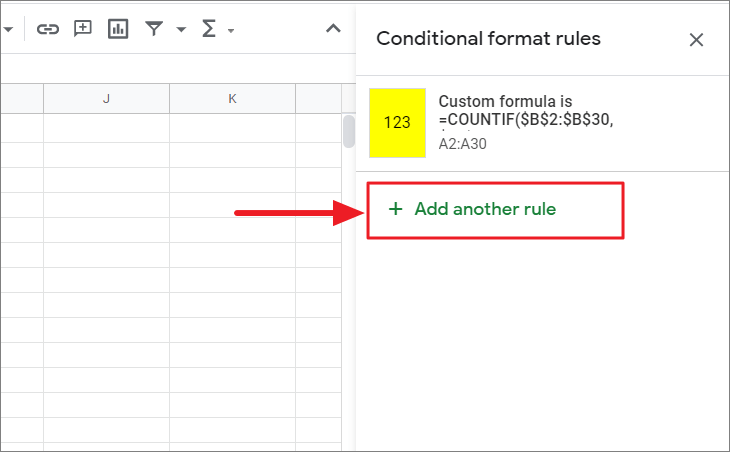
Now, we have to apply conditional formatting to Column B using the same formula. To do that, select the second column (B2:B30), go to the ‘Format’ menu, and select ‘Conditional formatting’.
Alternatively, click the ‘Add another rule’ button under the ‘Conditional format rules’ pane.
Next, confirm the range (B2:B30) in the ‘Apply to range’ box.
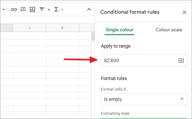
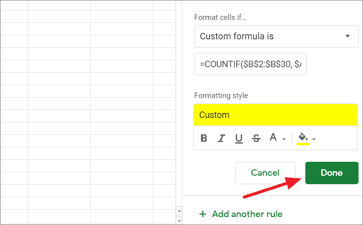
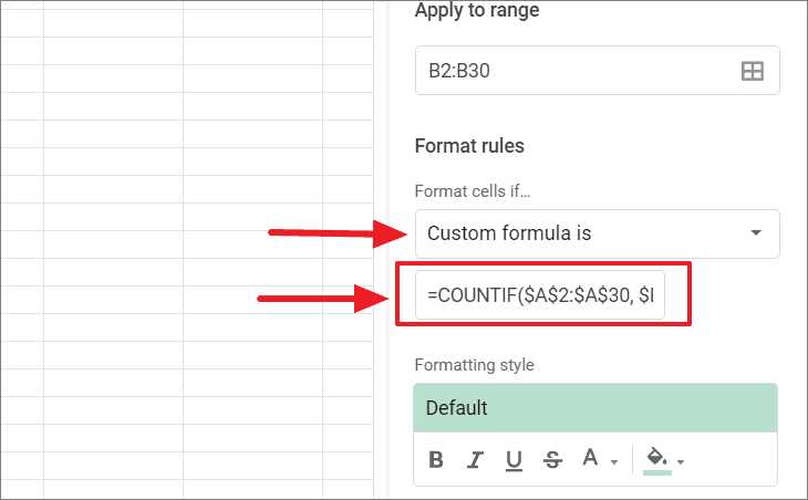
Then, set the ‘Format cells if..’ option to ‘Custom formula is’ and enter the below formula in the formula box:
=COUNTIF($A$2:$A$30, $B2)>0Here, we are using column A range ($A$2:$A$30) in the first argument and ‘$B2’ in the second argument. This formula will check the cell value in ‘column B’ against every cell in column A. If a match (duplicate) is found, then conditional formatting will hight that item in ‘column B’
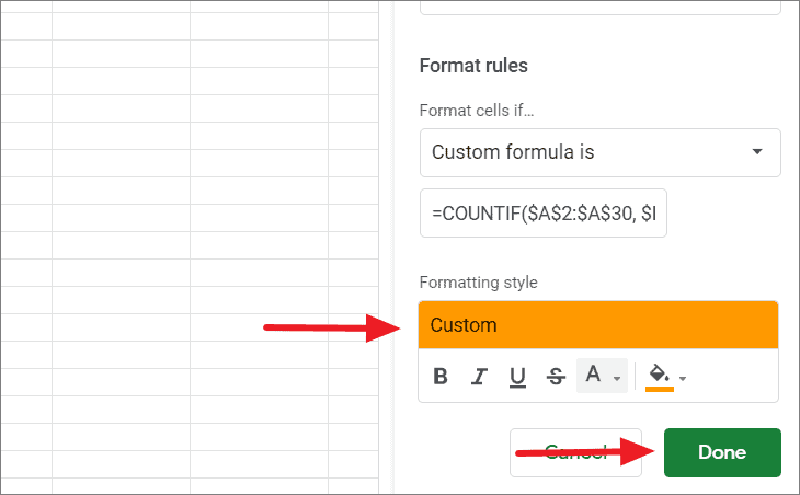
Then, specify the formatting in the ‘Formatting style’ options and click ‘Done’. Here, we’re choosing the orange color for column B.
This will highlight the column B items that have duplicates in column A. Now, you have found and highlighted duplicate items between two columns.
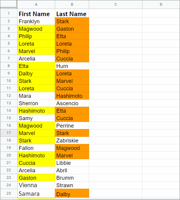
You probably noticed, although there is a duplicate for ‘Arcelia’ in column A, it is not highlighted. It is because the duplicatte value is only in one column (A) not between columns. Hence, it is not highlighted.
Highlight Duplicates Between Two columns in the Same Row
You can also highlight the rows that have the same values (duplicates) between two columns using conditional formatting. The conditional formatting rule can check each row and highlights the rows that have matching data in both columns. Here’s how you do this:
First, select both columns that you want to compare, then go to the ‘Format’ menu and select ‘Conditional formatting’.
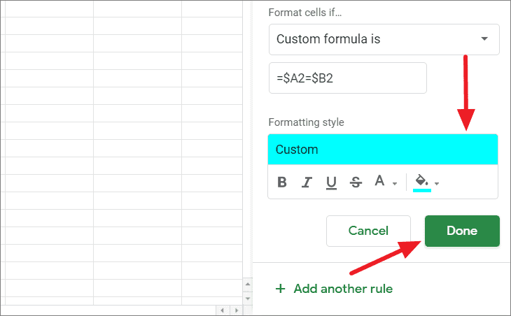
In the Conditional format rules pane, confirm the range in the ‘Apply to range’ box and choose ‘Custom formula is’ from the ‘Formula cells if..’ drop-down.
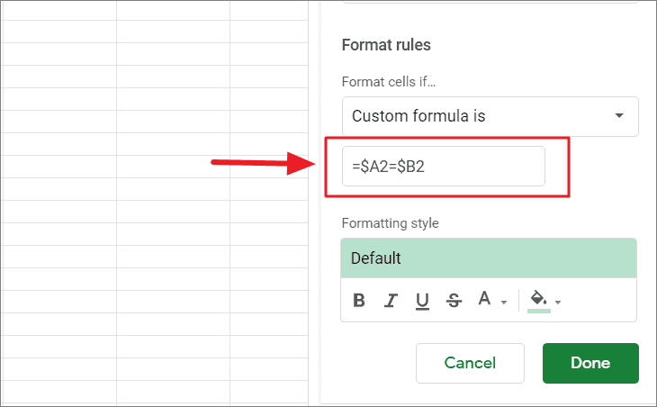
Then, enter the below formula in the ‘Value or formula’ box:
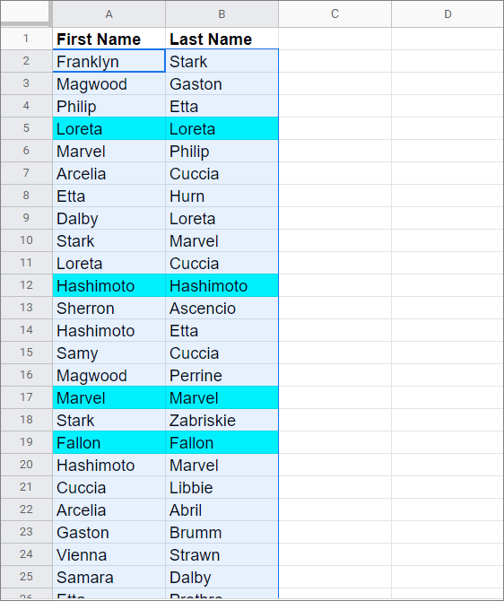
=$A2=$B2This formula will compare the two columns row-by-row and highlight rows that have identical values (duplicates). As you can see the formula entered here is only for the first row of the selected range, but the formula will be automatically applied to all the rows in the selected range by the conditional formating feature.
Then, specify the formatting from the ‘Formatting style’ options and click ‘Done’.
As you can see, only the rows that have matching data (duplicates) between two columns will be highlighted and all other duplicates will be ignored.
Highlight Duplicate Cells in Multiple Columns
When working with larger spreadsheets with many columns, you may want to highlight all the duplicates that appear across multiple columns instead of just one or two columns. You can still use conditional formatting to highlight the duplicate in multiple columns.
First, select the range of all columns and rows you want to search for duplicates instead of just one or two column. You can select entire columns by holding down the Ctrl key, then clicking on the letter at the top of each column. Alternatively, you can also click on the first and last cells in your range while also holding down the Shift key to select multiple columns at once.
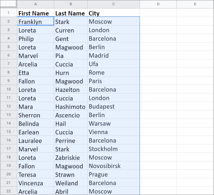
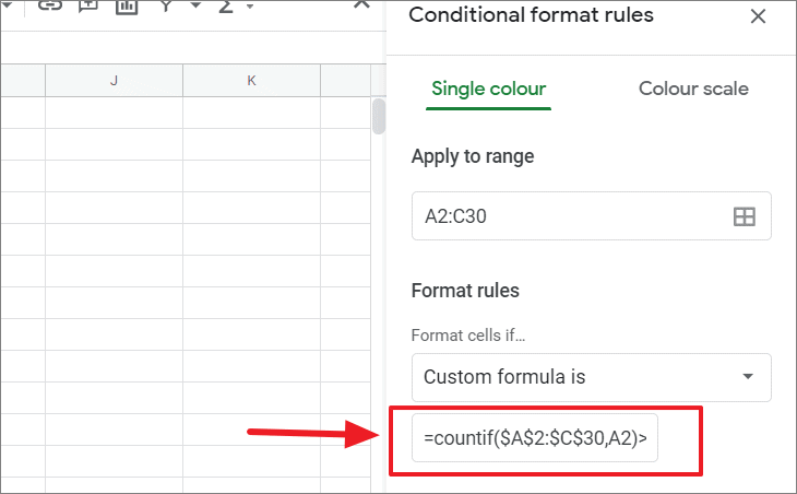
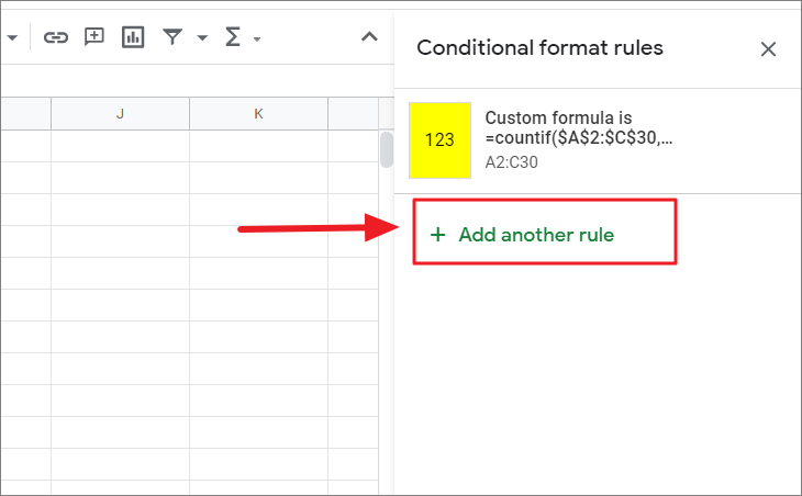
In the example, we are selecting A2:C30.
Then, click the ‘Format’ option in the menu and select ‘Conditional formatting’.
In the Conditional format rules, set the Format rules to ‘Custom formula is’, and then enter the following formula in the ‘Value or Formula’ box:
=countif($A$2:$C$30,A2)>We’re adding the ‘$’ sign before the cell references to make them absolute columns, so it doesn’t change we apply the formula. You can also enter the formula without the ‘$’ signs, it works either way.
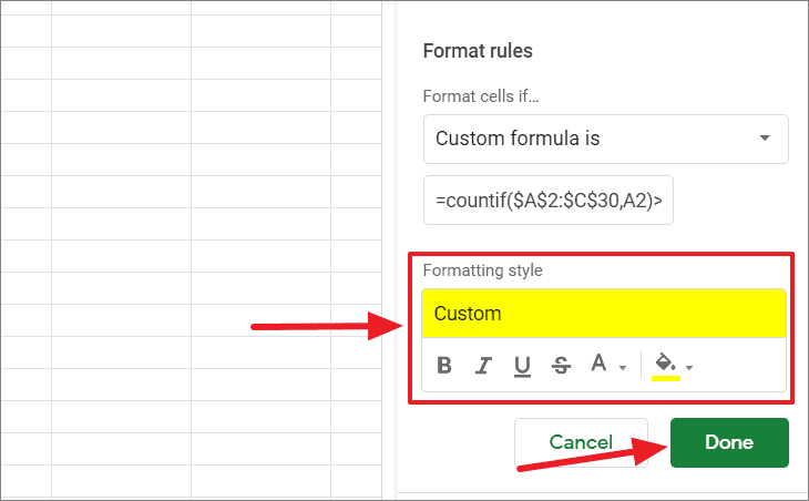
Then, choose the formatting in which you want to highlight the duplicate cells using the ‘Formatting style’ options. Here, we’re choosing ‘Yellow’ fill color. After that, click ‘Done’.
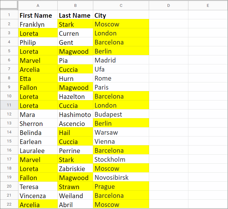
This will highlight the duplicates across all the columns you selected, as shown below.
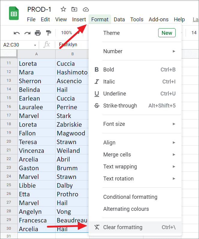
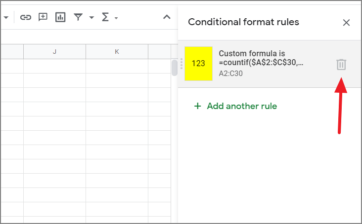
After applying the conditional formatting, you can edit or delete the conditional formatting rule anytime you want.
If you want to edit the current conditional formatting rule, select any cell with conditional formatting, go to ‘Format’ on the menu, and select ‘Conditional formatting’.
This will open the ‘Conditional format rules’ pane on the right with a list of format rules applied to the current selection. When you hover your mouse over the rule, it will show you the delete button, click on the delete button to remove the rule. Or, if you want to edit the rule that is currently showing, click on the rule itself.
If you want to add another conditional formatting over the current rule, click the ‘Add another rule’ button.
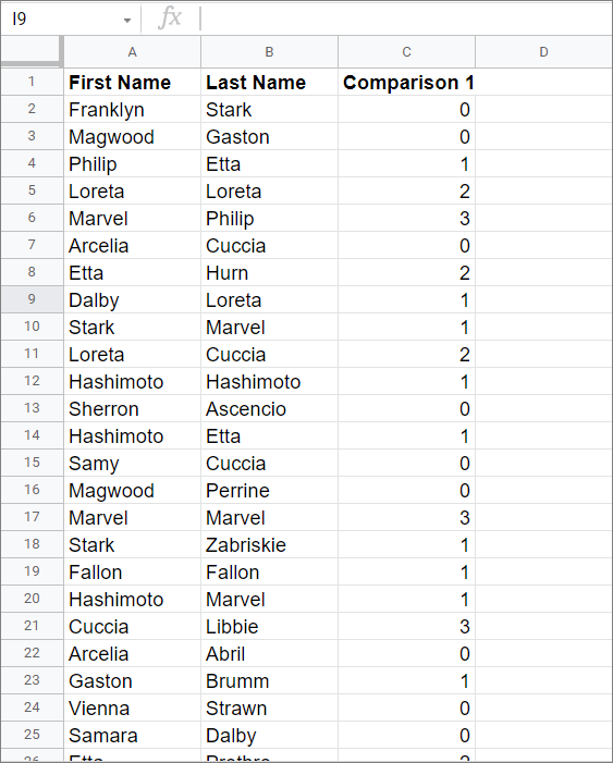
Count the Duplicates Between Two Columns
Sometimes, you want to count the number of times a value in one column repeats in another column. It can be easily done using the same COUNTIF function.
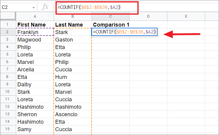
To find the number of times a value in column A exists in column B, enter the following formula in a cell in another column:
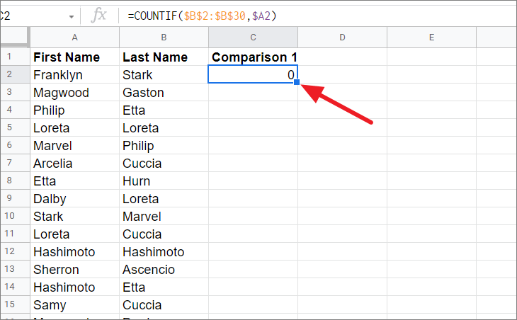
=COUNTIF($B$2:$B$30,$A2)Enter this formula in cell C2. This formula counts the number of times the value in cell A2 exists in the column (B2:B30) and returns the count in cell C2.
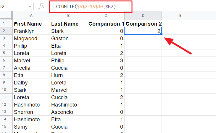
When you type the formula and press Enter, the Auto-Fill feature will appear, click the ‘Tick mark’ to auto-fill this formula to the rest of the cells (C3:C30).
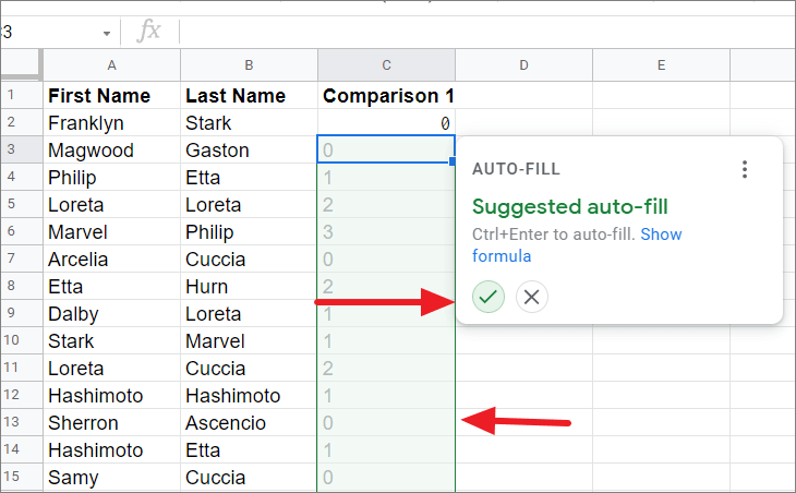
If the auto-fill feature doesn’t appear, click the blue square at the bottom-right corner of cell C2 and drag it down to copy the formula in cell C2 to cells C3:C30.
‘Comparison 1’ column (C) will now show you the number of times that each corresponding value in column A appears in column B. For example, the value of A2, or “Franklyn” is not found in column B, so, the COUNTIF function returns “0”. And the value “Loreta” (A5) is found twice in column B, hence, it returns “2”.
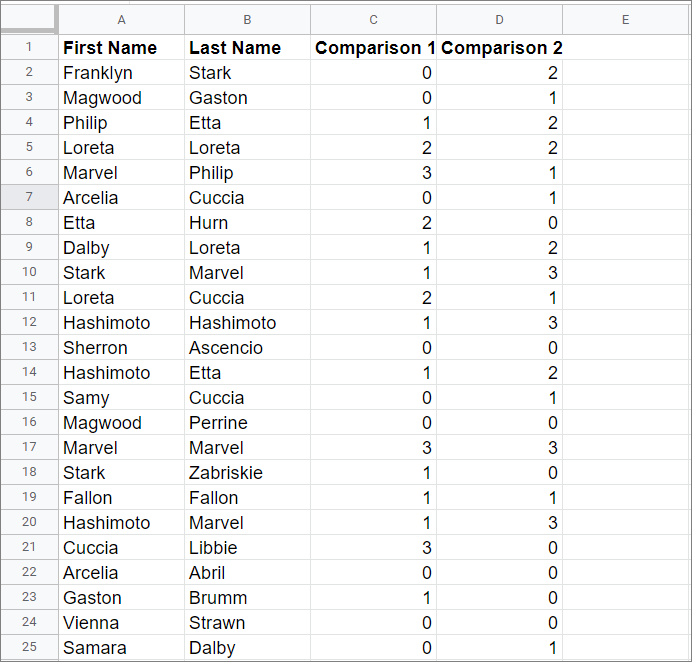
Now, we have to repeat the same steps to find the duplicate counts of column B. To do that, enter the following formula in cell D2 in column D (Comparison 2):
=COUNTIF($A$2:$A$30,$B2)In this formula, replace the range from ‘$B$2:$B$30’ to ‘$A$2:$A$30’ and ‘$B2’ to ‘$A2’. The function counts the number of times the value in cell B2 exists in the column A (A2:A30) and returns the count in cell D2.
Then, auto-fill the formula to the rest of the cells (D3:D30) in column D. Now, the ‘Comparison 2’ will show you the number of times that each corresponding value in column B appears in column A. For instance, the value of B2, or “Stark” is found twice in column A, so, the COUNTIF function returns “2”.
Note: If you want to count the duplicates across all columns or multiple columns, you just have to change the range in the first argument of the COUNTIF function to multiple columns instead of just one column. For example, change the range from A2:A30 to A2:B30, which will count the all the duplicates in two columns instead of just one.
That’s it.