
If you’ve been using Excel formulas for a while, you probably encountered the annoying #NAME? errors. Excel shows us this error to help us fix the problem with a formula, but it doesn’t exactly say what is really wrong with the formula.
The ‘#NAME?’ error appears in the cell when Excel doesn’t recognize your formula or arguments of your formula. It indicates that there is something is wrong or missing with the characters your formula used and that needs to be rectified.
There are several reasons why you would ever see the #NAME? errors in Excel. The common cause is the simple misspelling of the formula or function. But there are other reasons too including, incorrectly typed range name, misspelled cell range, missing quotation marks around the text in the formula, missing colon for a cell range, or incorrect formula version. In this article, we’ll explain some of the most common issues that can cause a #Name error in Excel and how to fix them.
Misspelled Formula or Function Name
The most common cause of #Name error is the misspelling of the function name or when the function doesn’t exist. When you entered an incorrect syntax of a function or formula, the #Name error is displayed in the cell where the formula is entered.
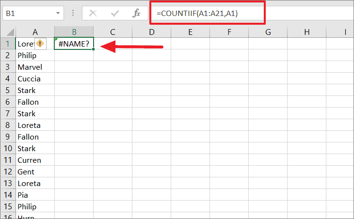
In the following example, the COUTIF function is used to count the number of times an item (A1) repeats in the list (column A). But, the function name “COUNIF” is misspelled as “COUNTIIF” with double ‘II’, hence the formula returns the #NAME? error.
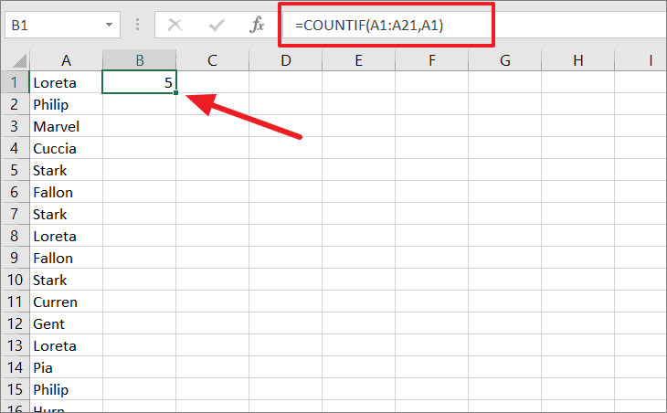
All you have to do is correct the spelling of the function, and the error is rectified.
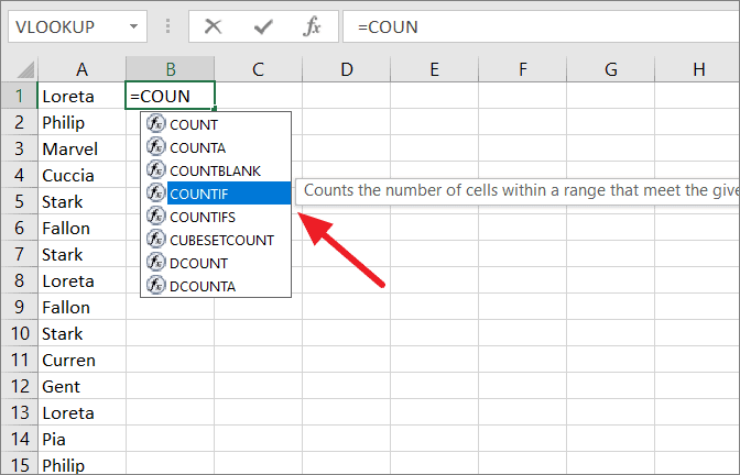
To avoid this error, you can use the formula suggestions rather than manually typing the formula. As soon as you start typing the formula, Excel will display a list of matching functions below where you’re typing as shown below.
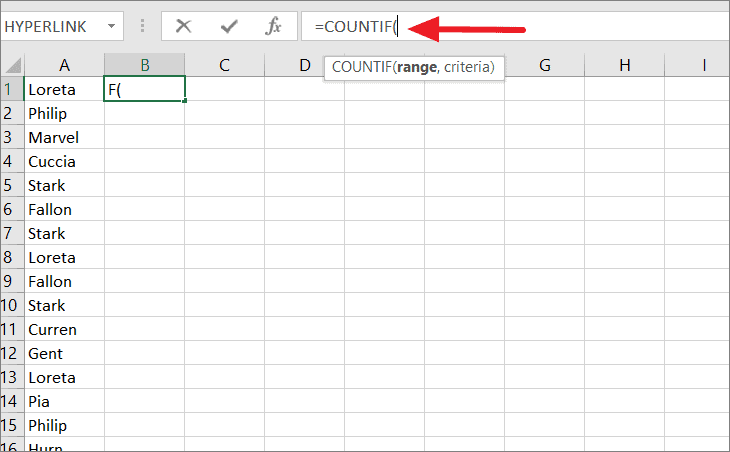
Double-click on one of the suggested functions or press TAB to accept a function suggested by autocomplete. Then, enter the arguments and press Enter.
Incorrect Cell Range
Another cause for the #Name error is because the cell range is entered incorrectly. This error will occur if you forget to include a colon (:) in a range or used the wrong combination of letters and numbers for the range.
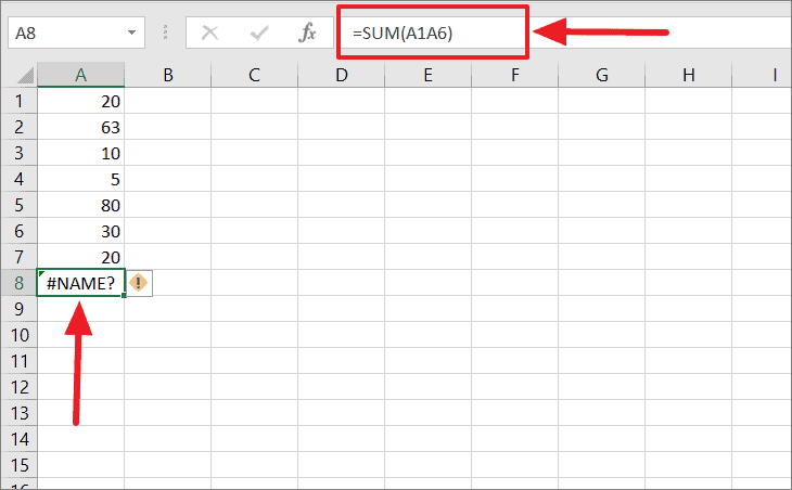
In the example below, the range reference is missing a colon (A1A6 instead of A1:A6), so the result returns the #NAME error.
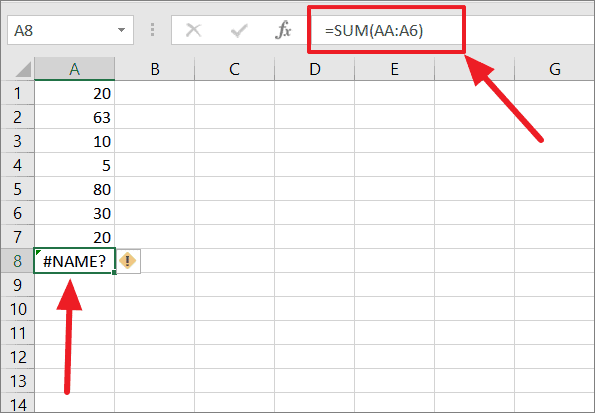
In the same example, the cell range has the wrong combination of letters and numbers, so it returns the #NAME error.
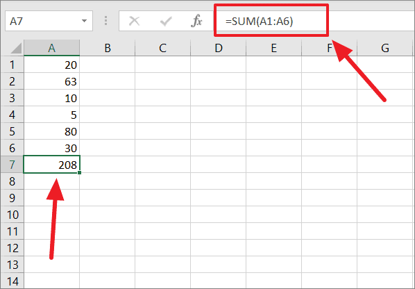
Now, the range used in cell A7 has been fixed to get the proper result:
Misspelled Named Range
A named range is a descriptive name, used to refer to individual cells or range of cells instead of the cell address. If you misspell a named range in your formula or refer to a name that is not defined in your spreadsheet, then the formula will generate the #NAME? Error.
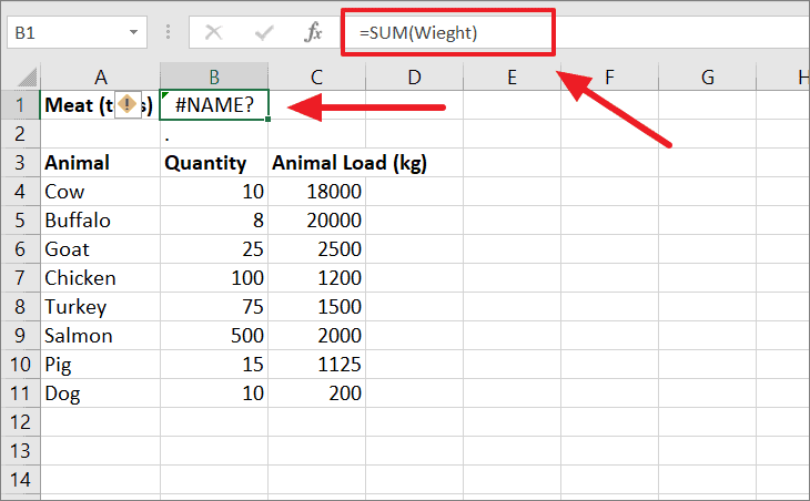
In the below example, the range C4:C11 is named “Weight”. When we try to use this name to sum the range of cells, we get the #Name? error. It’s because the range name “Weight” is misspelled “Wieght” and the SUM function in B2 returns the #NAME? error.
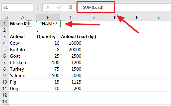
Here, we get the #Name error, because we tried to use the undefined named range “Load” in the formula. The named range “Load” doesn’t exist in this sheet, so we got the #NAME error.
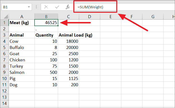
Below, correcting the spelling of the defined cell range fixes the issue and returns the ‘46525’ as the total weight of the Meat.
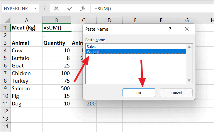
To avoid this error, you can use the ‘Paste Name’ dialog box to insert the name of the range into the function instead of typing the name. When you need to type the name of the range within your formula, press the F3 function key to see the list of named ranges in your workbook. On the Paste Name dialog box, select the name and click ‘OK’ to automatically insert a named range into the function.
This way you don’t have to manually type the name which prevents the error from happening.
Check the Scope of Named Range
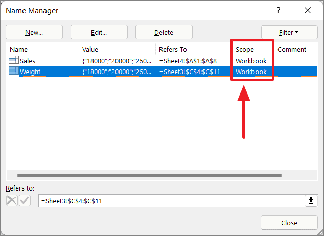
Another reason you might get a ‘#NAME?’ error is when you try to reference a locally scoped named range from another worksheet within the workbook. When you are defining a named range, you can set whether you want the scope of the named range to the whole workbook or only to a particular sheet.
If you have set the scope of the named range to a particular sheet and try to reference it from a different worksheet, you will see the #NAME? Error.
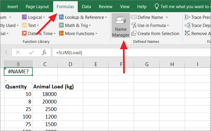
To check the scope of the named ranges, click the ‘Name Manager’ option from the ‘Formula’ tab or press Ctrl + F3. It will show you all the named ranges and table names in the workbook. Here, you can create, delete or edit the existing names.
Although you can check the scope of the named ranges in the ‘Name Manager’ dialog box, you can’t change it. You can only set the scope when creating a named range. Correct the named range accordingly or define a new named range to fix the issue.
Text Without Double Quotes (” “)
Entering a text value without double quotes in a formula will also cause the #NAME Error. If you enter any text values in the formulas, you must enclose them in double quotation marks (” “), even if you’re only using a space.
For example, the formula below is trying to look up the quantity of ‘Pig’ in the table using the VLOOKUP function. But, in B13, the text string ‘Pig’ is entered without double quotes (“ “) in the formula. So the formula returns the #NAME? error as shown below.
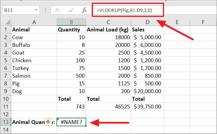
If there are quotes around a value, Excel will treat it as a text string. But when a text value is not enclosed in double-quotes, Excel considers it as a named range or formula name. When that named range or function is not found, Excel returns the #NAME? error.
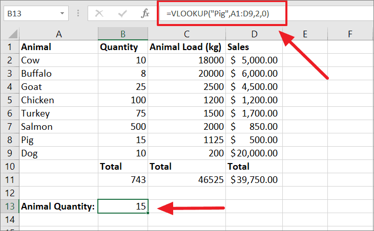
Just enclose the text value “Pig” in double-quotes in the formula and the #NAME error will disappear. After quotes have been added, the VLOOKUP function returns the Pig’s quantity as ’15’.
Note: The text value needs to be enclosed with straight double quotes (i.e. “Dog”). If you enter a text value with smart quotes (i.e. ❝Dog❞), Excel won’t recognize these as quotes and will instead result in the #NAME? error.
Using New Version Formulas in Older Excel Versions
The functions that were introduced in the new Excel version don’t work on older Excel versions. For instance, new functions such as CONCAT, TEXTJOIN, IFS, SWITCH, etc. were added in Excel 2016 and 2019.
If you try to use these new functions in older Excel versions like Excel 2007, 2010, 2013 or open a file that contains these formulas in an older version, you’ll probably get a #NAME error. Excel doesn’t recognize these new functions because they don’t exist in that version.
Sadly, there is no fix to this issue. You simply can’t use the newer formulas in an older version of Excel. If you are opening a workbook in an older version, make sure you don’t include any of the newer functions in that file.
Also, If you save a workbook that has a macro with a formula using the ‘Save As’ option, but you didn’t enable the macros in the newly saved file, you’ll likely see a #NAME error.
Finding all #NAME? Errors in Excel
Let’s say you receive a large spreadsheet from a colleague and you’re not able to perform some calculations due to errors. If you don’t know where all of your errors lie, there are two different ways you can use to find #NAME errors in Excel.
Using the Go To Special Tool
If you want to find any and all errors in your worksheet, you can do so with the Go To Special feature. The Go To Special Tool finds not only the #NAME? errors but all kinds of errors in a spreadsheet. Here’s how you do this:
Open the spreadsheet in which you want to select the cells with error, then, click on the ‘Find and Select’ icon in the Editing group of the ‘Home’ tab.
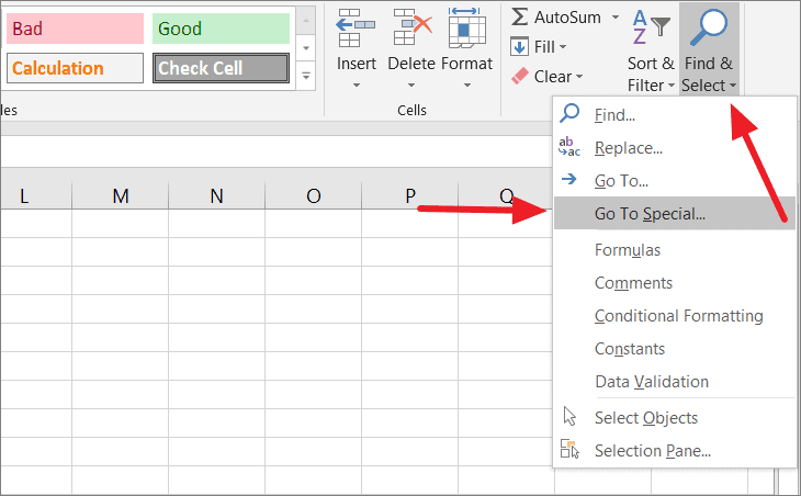
Alternatively, press F5 open the ‘Go To’ dialog and click the ‘Special’ option.
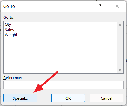
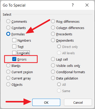
Either way, it will open the ‘Go to Special’ dialog box. Here, choose the ‘Formulas’ option, deselect all the other options under Formulas and then, leave the box that says ‘Errors’ selected. Then, click ‘OK’.
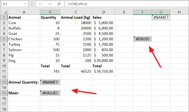
This will select all the cells that have any kind of error in them as shown below. After the error cells are selected, you can then treat them however you want.
Using Find and Replace
If you only want to find out the #NAME errors in the sheet, you can use the Find and Replace tool. Follow these steps:
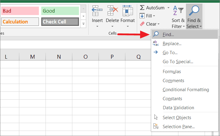
First, select the range or select the entire worksheet (by pressing Ctrl + A) in which you want to find the Name error. Then, click ‘Find & Select’ in the ‘Home’ tab and select ‘Find’ or press Ctrl + F.
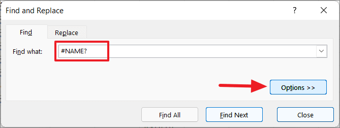
In the Find and Replace dialog box, type #NAME? in the ‘Find what’ field and click the ‘Options’ button.
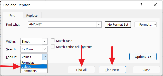
Then, choose ‘Values’ in the ‘Look in’ drop-down, and then choose either ‘Find Next’ or ‘Find All’.
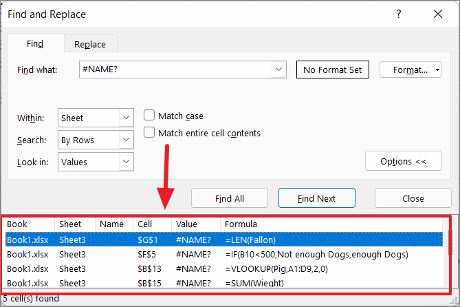
If you select ‘Find Next’, Excel selects the cells one by one that has the Name error which can be treated individually. Or, if you select ‘Find All’, another box will appear under the Find and Replace dialog that lists all the cells with the #NAME errors.
Avoiding #NAME? Errors in Excel
We have seen the most common cause of #NAME errors in Excel and how to fix and avoid them. But the best way to prevent the #NAME errors is to use the Function Wizard to enter formulas in the sheet.
Excel Function Wizard allows you to quickly generate valid functions. It provides you with a list of functions with syntax (range, criteria) which you can easily implement. Here’s how:
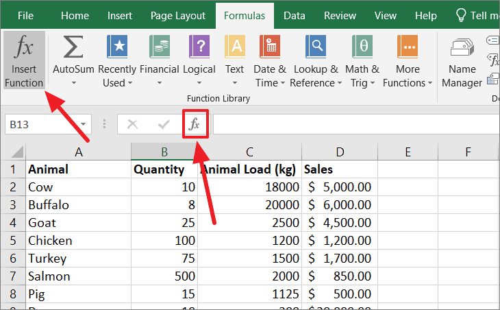
First, select the cell where you want to insert the formula. Then, you can either go to the ‘Formulas’ tab and click the ‘Insert Function’ option on the Function Library group or you can click on the Function Wizard button ‘fx’ located on the toolbar next to the formula bar.
You can also choose a function from any one of the categories available in the ‘Function Library’ under the ‘Formulas’ tab.
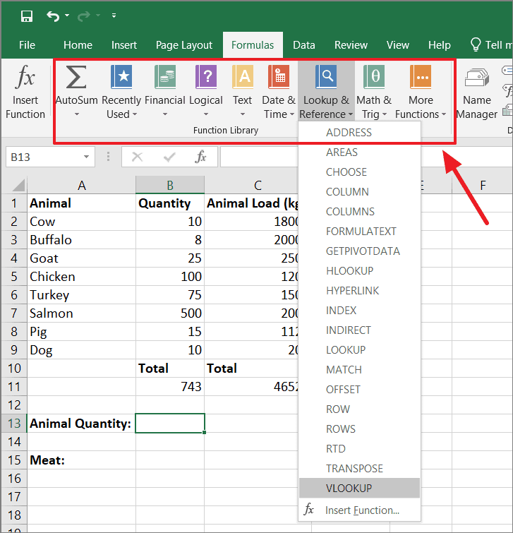
In the Insert Function dialog box, click on the drop-down menu next to ‘select a category’ and pick one of the 13 categories listed there. All the functions under the selected category will be listed in the ‘Select a function’ box. Select the function you want to insert and click ‘OK’
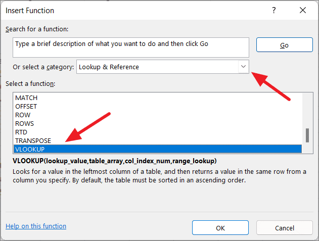
Alternatively, you can type the formula (you can also type a partial name) in the ‘Search for a function’ field and search for it. Then, double-click on the function or click ‘OK’.

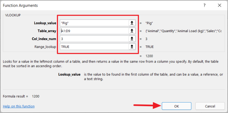
This will open up the Function Arguments dialog box. Here, you need to enter the function’s arguments. For example, we want to look up the quantity of the ‘Pig’ in the table using the VLOOKUP function.
The Look_value is entered ‘Pig’. For Table_array, you can directly enter the range of the table (A1:D9) in the field or click the upward arrow button inside the field to select the range. Co_index_num is entered ‘3’ and Range_lookup is set to ‘TRUE’. Once, you have specified all the arguments, click the ‘OK’ button.
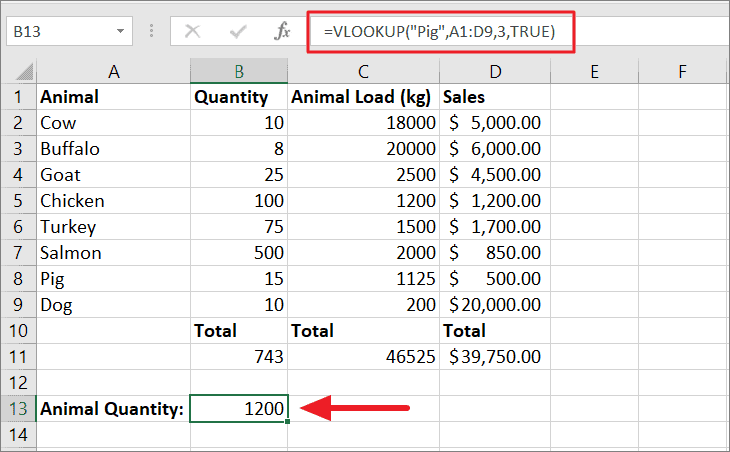
You will see the result in the selected cell and the completed formula in the Formula bar.
Using the Formula Wizard can save you a lot of time and help you avoid the #NAME? errors in Excel.
That’s it.


