How to Freeze Panes in Excel

Working with extensive data in Excel often requires scrolling, which can cause important headers or labels to disappear from view. Freezing panes keeps specific rows or columns visible, enhancing navigation and ensuring critical information remains accessible as you scroll through your worksheet.

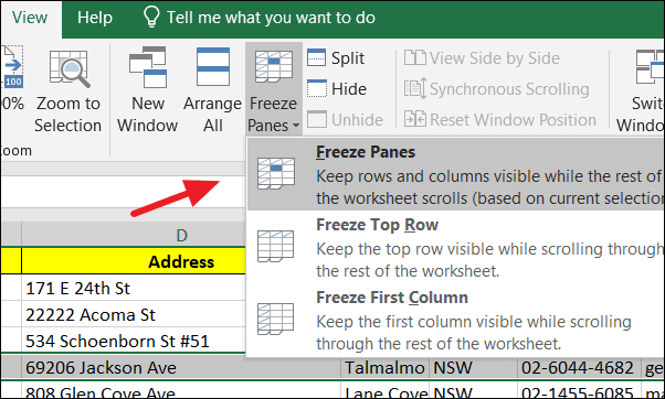
How to freeze rows and columns together

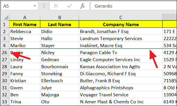
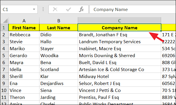
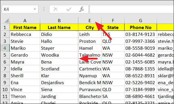
To keep both specific rows and columns visible while scrolling, you can freeze them simultaneously. Follow these steps:

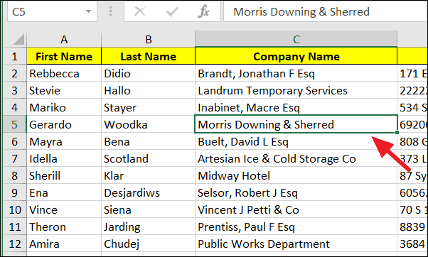
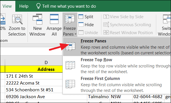
Click on the cell immediately below the last row and to the right of the last column you want to keep visible. For example, if you wish to freeze the first four rows and the first two columns, select cell C5.

Go to the View tab on the Ribbon. Click on Freeze Panes in the Window group, and select Freeze Panes from the dropdown menu.

Now, both the specified rows and columns will remain visible as you scroll through the worksheet.

How to freeze the top row

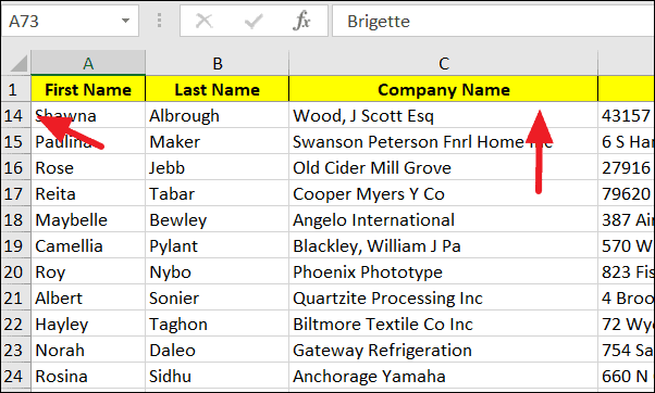
Keeping the header row visible is crucial when working with long lists of data. To freeze the top row:

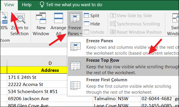
Navigate to the View tab on the Ribbon.

Click on Freeze Panes and select Freeze Top Row from the dropdown menu.

The first row will now remain visible as you scroll down the worksheet.

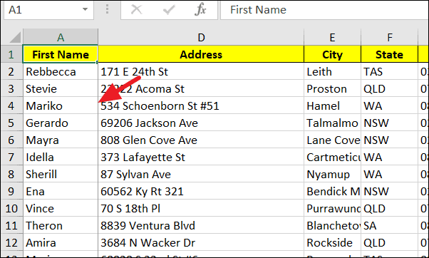
How to freeze the first column

If you need to keep the first column in view while scrolling horizontally, follow these steps:

Go to the View tab on the Ribbon.

Click on Freeze Panes and choose Freeze First Column from the dropdown menu.

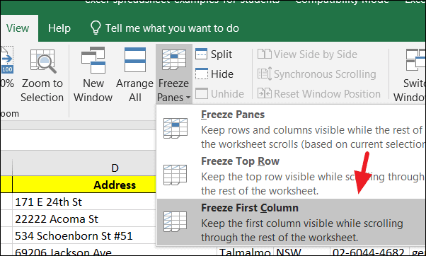
The first column will stay visible as you scroll to the right.

How to freeze multiple rows

To freeze multiple rows at the top of your worksheet:

Select the row immediately below the last row you want to freeze. For example, to freeze the first four rows, select row 5.

Navigate to the View tab, click on Freeze Panes, and select Freeze Panes from the dropdown menu.

A thin line will appear below the frozen rows, indicating that they will remain visible as you scroll.

How to freeze multiple columns

To keep multiple columns visible while scrolling horizontally:

Select the column immediately to the right of the last column you want to freeze. For instance, to freeze the first two columns, select column C.

Go to the View tab, click on Freeze Panes, and select Freeze Panes from the dropdown menu.

The selected columns will now remain visible as you scroll to the right.

How to unfreeze rows or columns

If you need to unfreeze panes to reset or change which rows or columns are frozen:

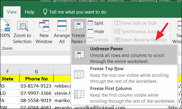
Navigate to the View tab on the Ribbon.

Click on Freeze Panes and select Unfreeze Panes from the dropdown menu.

This will release all frozen panes, allowing you to set new ones as needed.

Freezing panes in Excel enhances your ability to navigate and analyze large datasets by keeping essential information in view. Utilize these methods to improve your workflow and data management.