
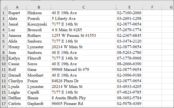
In Excel, dealing with large datasets can be challenging, especially when duplicate entries affect data accuracy and analysis. Duplicate values can lead to misleading results, making it crucial to identify and highlight them effectively.
Excel provides several methods to highlight duplicate values, ensuring that you can spot and address them promptly. This guide covers the most efficient techniques to highlight duplicates using Excel’s built-in Conditional Formatting feature and custom formulas.
Highlight Duplicates with Conditional Formatting’s Duplicate Values Rule
The simplest way to highlight duplicates in Excel is by using the built-in Duplicate Values rule in Conditional Formatting. Here’s how to do it:
Home tab on the Excel ribbon. In the Styles group, click on Conditional Formatting. Hover over Highlight Cells Rules and select Duplicate Values from the submenu.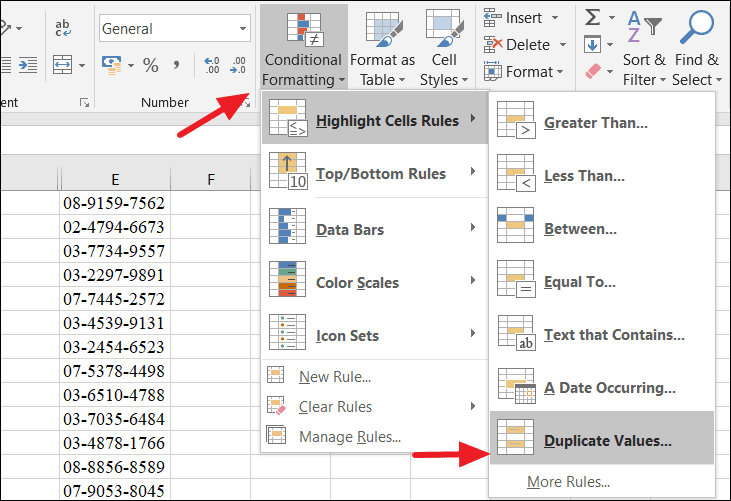
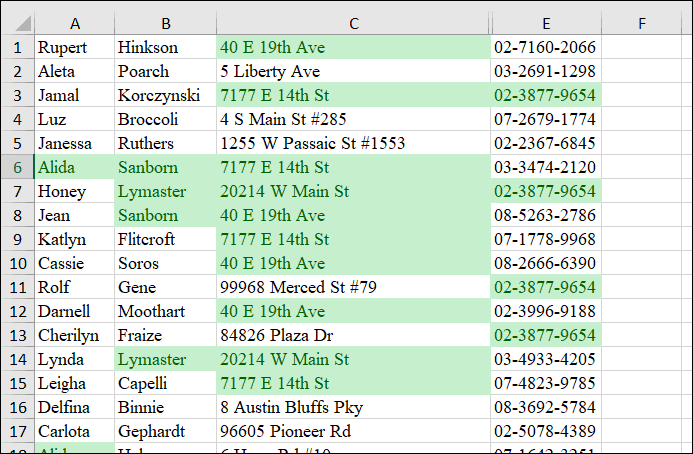
Green Fill with Dark Green Text. Click OK to apply the formatting.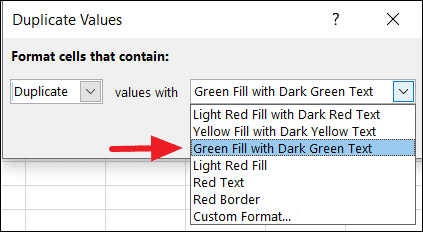
Highlight Duplicates Using a COUNTIF Formula with Conditional Formatting
For more advanced control, you can use a custom COUNTIF formula within Conditional Formatting to highlight duplicates. This method is particularly useful when dealing with duplicates across multiple columns or when you need specific criteria.
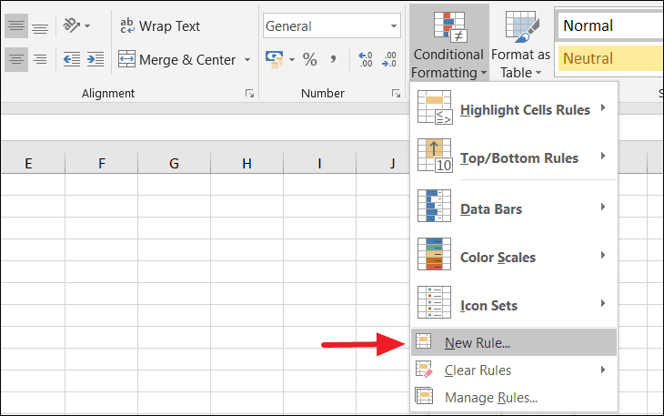
Home tab, click on Conditional Formatting, and choose New Rule from the dropdown menu.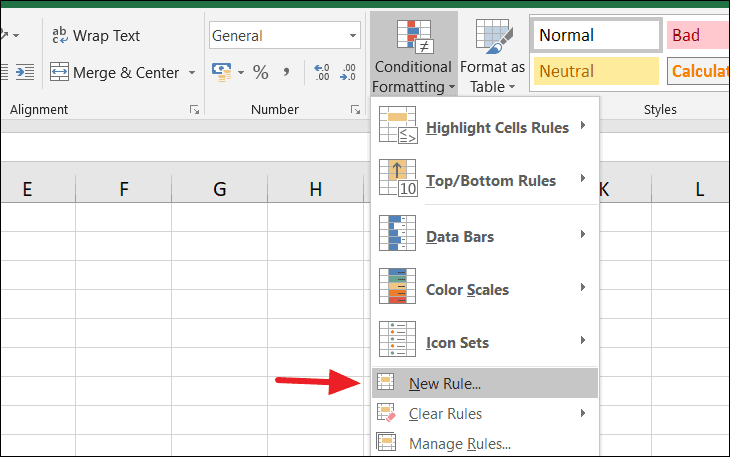
=COUNTIF($A$1:$C$11,A1)>1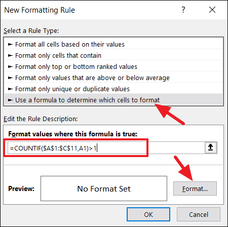
This formula counts how many times each value appears in the range A1:C11. If a value appears more than once, it is considered a duplicate.
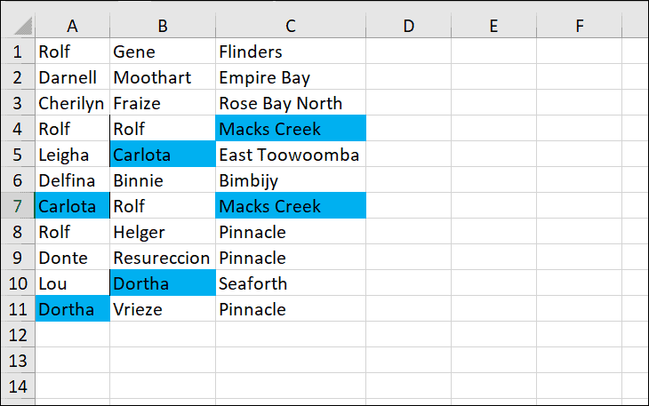
Format button to specify how you want to highlight the duplicates. In the Format Cells dialog, choose a fill color or any other formatting style you prefer. Here, we’ll select a blue fill color. Click OK to confirm.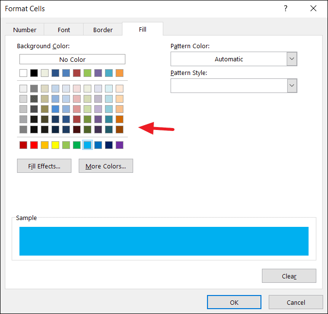
OK again to apply the conditional formatting rule. The duplicates in your selected range will now be highlighted using the formatting you specified.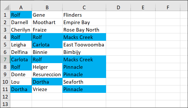
Note: Always write the formula relative to the first cell in your selected range (e.g., A1). Excel adjusts the formula for other cells automatically.
You can customize the formula to meet different criteria. For example, to highlight values that appear exactly twice, use:
=COUNTIF($A$1:$C$11,A1)=2This formula will only highlight cells that have duplicates appearing exactly two times.
Home tab, click on Sort & Filter, and choose Filter.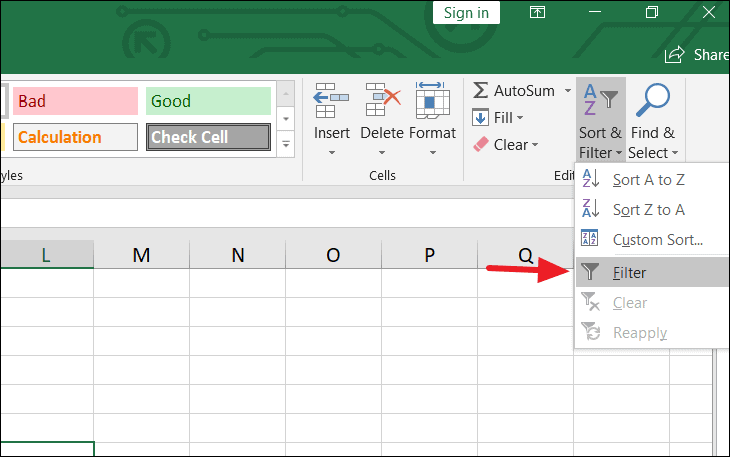
Filter by Color, and select the color used to highlight the duplicates (e.g., blue).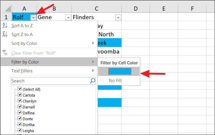
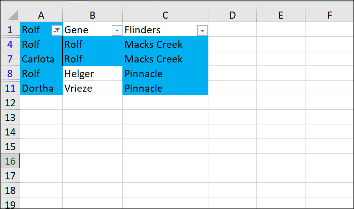
This will display only the duplicate entries, allowing you to focus on them exclusively.
Highlight Duplicate Rows Using COUNTIFS Formula
To find and highlight duplicate rows (where all cells in a row are identical to another row), use the COUNTIFS function within Conditional Formatting.
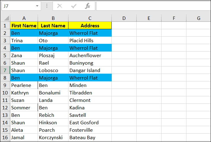
=COUNTIFS($A$1:$A$20,$A1,$B$1:$B$20,$B1,$C$1:$C$20,$C1)>1This formula checks for duplicate rows based on the columns specified (A, B, and C). It counts the number of times the combination of values in each row appears in the dataset.
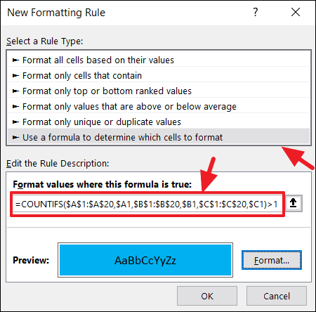
Format to choose your desired formatting for duplicate rows. After selecting the format, click OK to apply the rule.Excel will now highlight the duplicate rows in your dataset, allowing you to identify and address them accordingly.
By leveraging Excel’s Conditional Formatting with built-in rules and custom formulas, you can efficiently highlight duplicate values and rows, ensuring data integrity and accuracy in your spreadsheets.


