The font strikethrough option isn’t readily available on the ribbon, but there are various ways to access the strikethrough effect in Excel.
The font strikethrough option isn’t readily available on the ribbon, but there are various ways to access the strikethrough effect in Excel.
by Raj Kumar
Strikethrough formatting in Excel allows you to draw a line through text, indicating revisions or completed tasks. Although Excel doesn’t provide a direct strikethrough button on the ribbon by default, there are several ways to apply this formatting to your cells.
Add a strikethrough button to the quick access toolbar
Adding a strikethrough button to the Quick Access Toolbar (QAT) provides quick access to this formatting option with a single click.
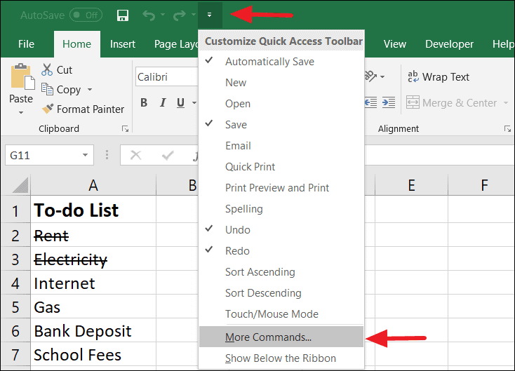
Click the small downward arrow in the upper left corner of the Excel window to open the Quick Access Toolbar customization menu. From the drop-down menu, select ‘More Commands…’.
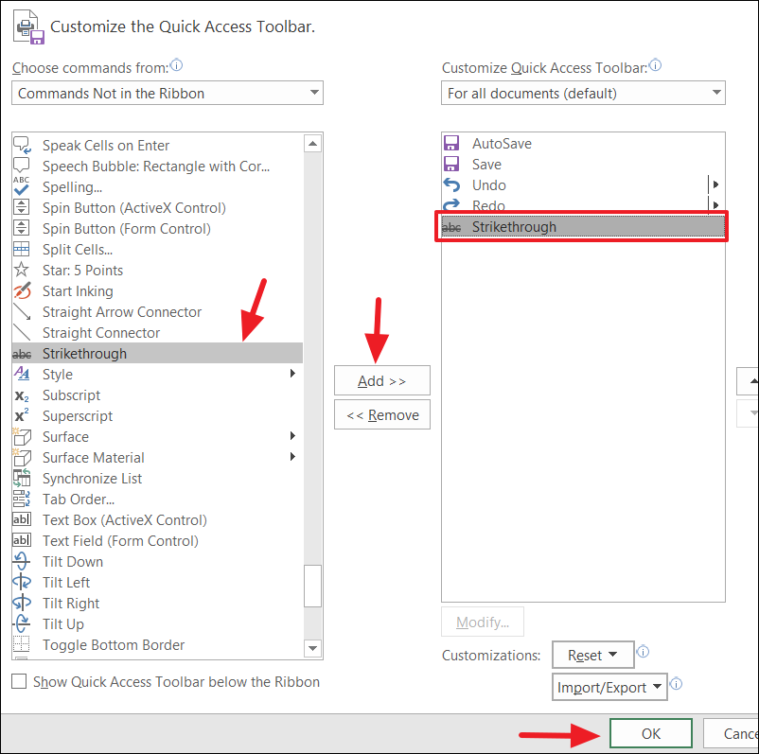
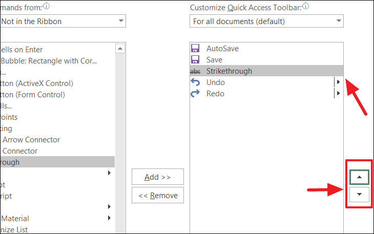
Use the up and down arrow buttons on the right side of the dialog box to position the strikethrough button where you prefer on the toolbar. Click ‘OK’ to save the changes and close the dialog box.
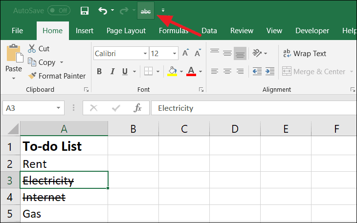
The strikethrough button will now appear in the Quick Access Toolbar at the top of your Excel window.
To use the strikethrough button, select the cell or text you want to format and click the strikethrough icon on the Quick Access Toolbar.
Apply strikethrough using a keyboard shortcut
Using a keyboard shortcut is a fast way to apply strikethrough formatting without navigating through menus.
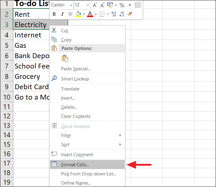
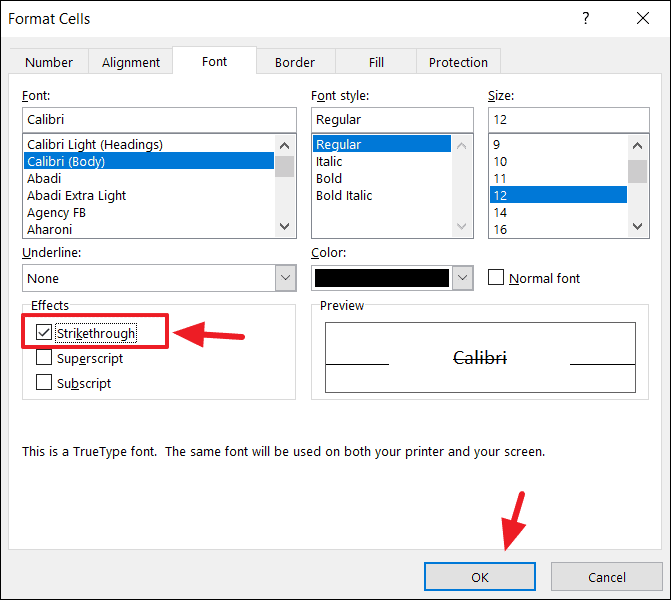
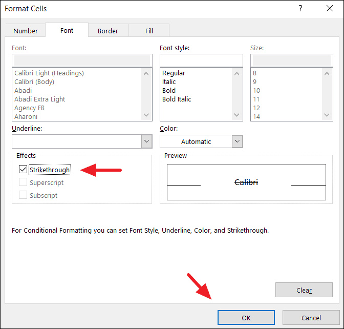
In the Format Cells dialog, navigate to the ‘Font’ tab. Under the ‘Effects’ section, check the box next to ‘Strikethrough’. Click ‘OK’ to apply the formatting.
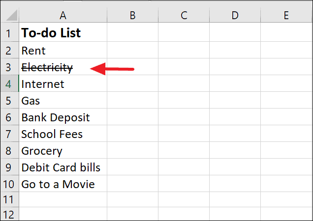
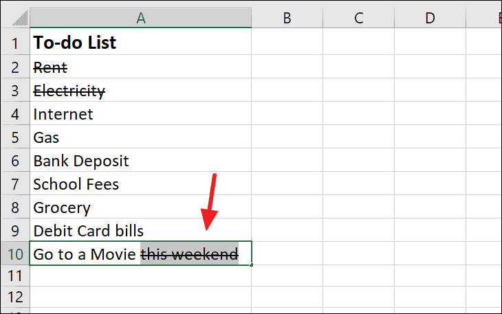
The selected text will now appear with a line through it.
Add a strikethrough button to the ribbon
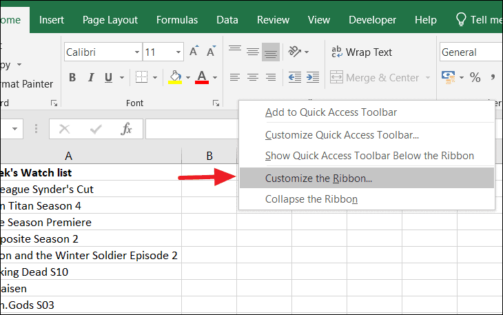
Customizing the Excel ribbon to include a strikethrough button can make this formatting option more accessible.
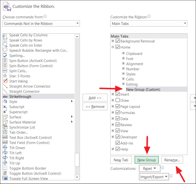
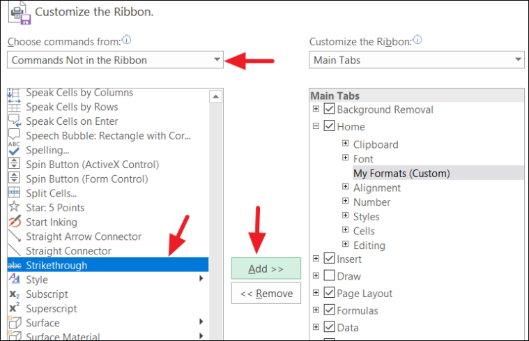
In the Excel Options window, select the tab where you want to add the strikethrough button, such as the ‘Home’ tab. Click the ‘New Group’ button to create a custom group.
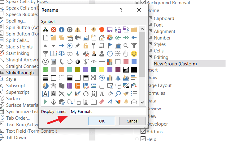
With the new group selected, click ‘Rename’ to give it a descriptive name, like ‘My Formats’. Enter the name in the ‘Display name’ field and click ‘OK’.
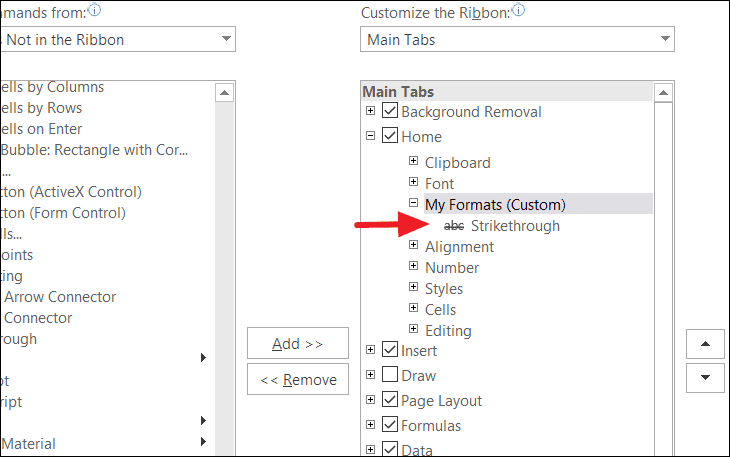
Click the ‘Add’ button to include the strikethrough command in your custom group. Use the up and down arrow buttons to position the group where you want it on the ribbon. Click ‘OK’ to save the changes.
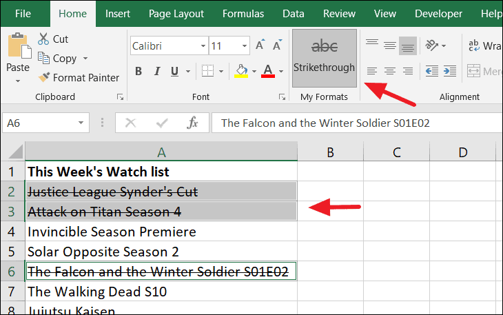
The strikethrough button will now appear in your specified tab and group on the ribbon.
To use it, select the cells you want to format and click the strikethrough button on the ribbon.
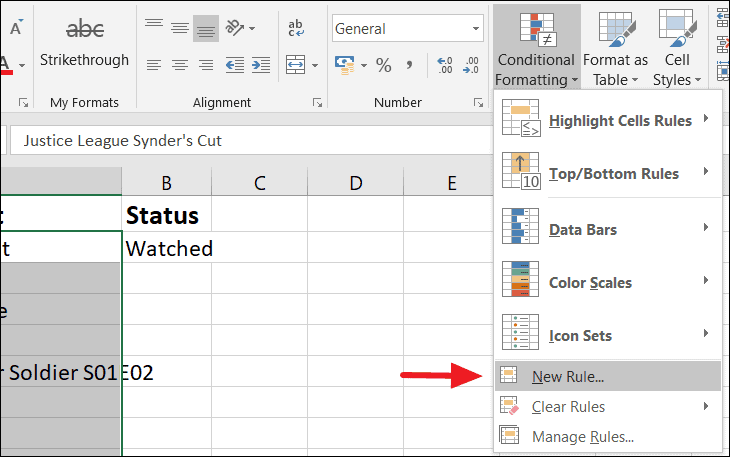
Apply strikethrough using conditional formatting
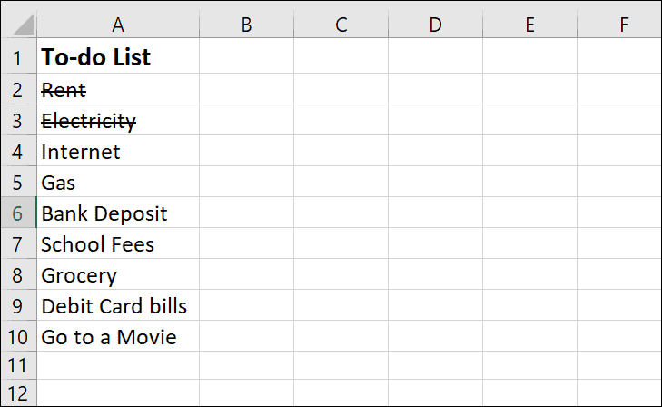
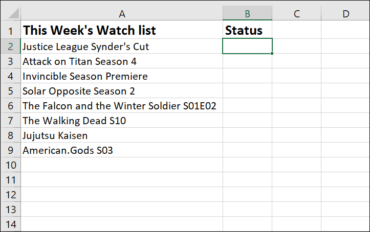
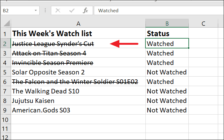
Conditional formatting can automatically apply strikethrough formatting based on specific criteria, such as marking tasks as completed.
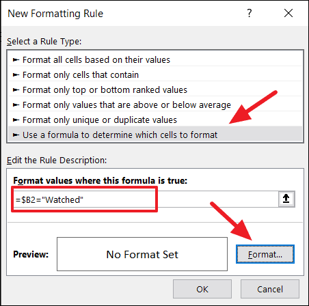
In the New Formatting Rule dialog box, select ‘Use a formula to determine which cells to format’. Enter the following formula in the ‘Format values where this formula is true’ field:
Click ‘Format…’ to open the Format Cells dialog. Navigate to the ‘Font’ tab and check the ‘Strikethrough’ option under the ‘Effects’ section. Click ‘OK’ to close both dialog boxes and apply the rule.
Now, when you update the status to ‘Watched’ in column B, the corresponding cell in column A will automatically display the strikethrough formatting.
These methods offer various ways to apply strikethrough formatting in Excel, whether through quick shortcuts, toolbar buttons, or automated rules, enhancing your ability to manage and present data effectively.