How to Insert Check Mark (Tick) in Excel

Excel spreadsheets often benefit from visual indicators like check marks to denote completed tasks, affirmative responses, or correct entries. While these symbols are sometimes confused with interactive checkboxes, they are actually static characters inserted into cells. This guide will walk you through several methods to add check marks to your Excel worksheets, enhancing your data presentation and list management capabilities.

Using the Symbol dialog box

One of the most versatile ways to insert a check mark is through the Symbol dialog box:

1. Click on the cell where you want to add the check mark.
2. Navigate to the 'Insert' tab in the Excel ribbon.
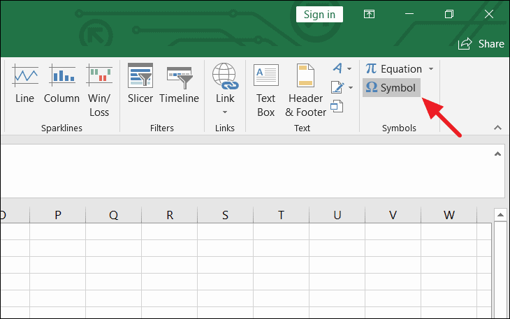
3. Find the 'Symbols' group and click on 'Symbol'.

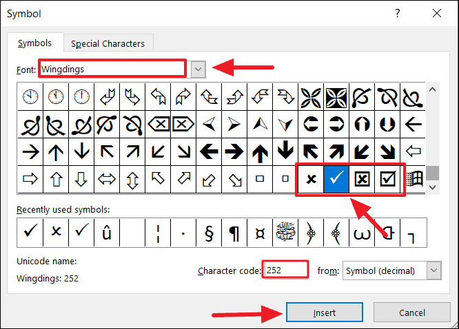
4. In the Symbol dialog box, select 'Wingdings' from the Font dropdown menu.
5. Scroll through the symbols to find various check mark options.
6. Choose your preferred check mark and click 'Insert'.

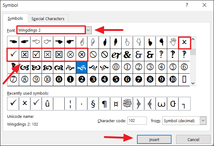
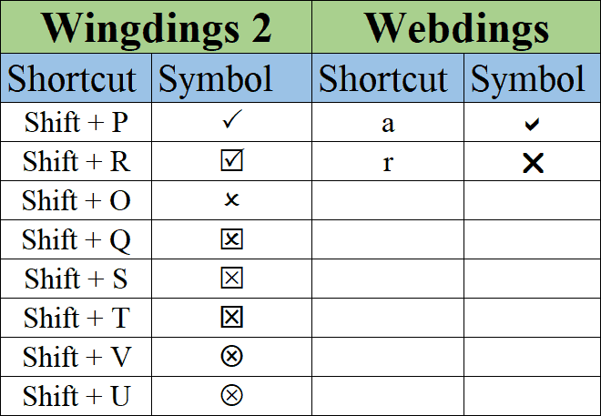
For additional options, you can also try the 'Wingdings 2' font:

7. Click 'Close' when you're finished.

Keyboard shortcuts

A quick method for inserting check marks involves using keyboard shortcuts:

1. Select the cell where you want the check mark.
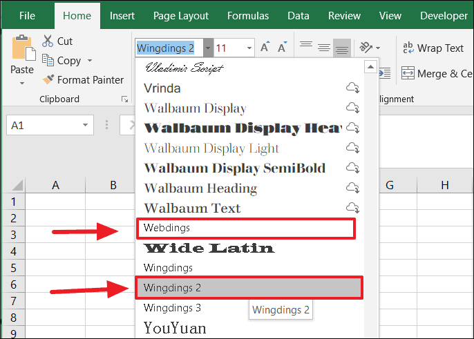
2. Go to the 'Home' tab and change the font to 'Wingdings 2' or 'Webdings'.

3. Use these keyboard combinations to insert various symbols:

CHAR function

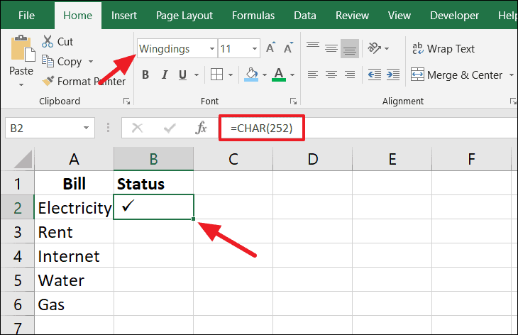
Excel's CHAR function allows you to insert symbols programmatically:

1. In your desired cell, enter the formula: =CHAR(character code)
2. Replace 'character code' with the appropriate number (e.g., 252 for a check mark).
3. Ensure the cell's font is set to 'Wingdings' to display the symbol correctly.

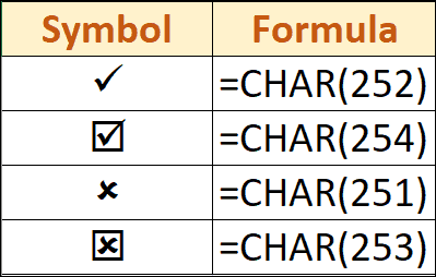
Here are some common character codes for check marks and cross marks:

Alt codes

For swift check mark insertion using Alt codes:

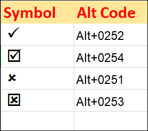
1. Set the cell font to 'Wingdings'.
2. Hold down the Alt key and type these codes on the numeric keypad:

AutoCorrect feature

Customize Excel's AutoCorrect feature for rapid check mark insertion:

1. Insert a check mark using any previous method.
2. Copy the check mark from the formula bar.
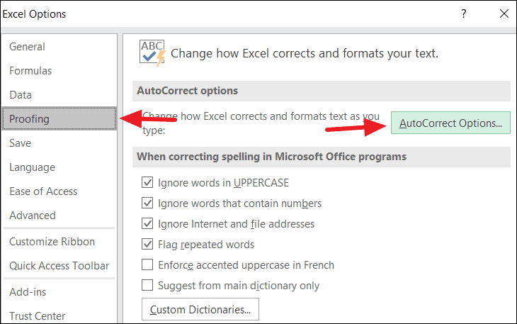
3. Navigate to File > Options > Proofing > AutoCorrect Options.

4. In the AutoCorrect dialog box:
   • Type a shortcut (e.g., 'chk') in the 'Replace' field.
   • Paste the copied check mark in the 'With' field.
   • Click 'Add', then 'OK'.

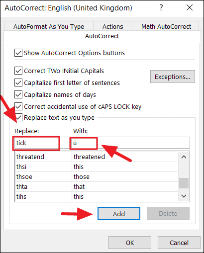
Now, typing 'chk' in a cell will automatically insert the check mark symbol. Remember to set the cell font to 'Wingdings' for proper display.

Copy and paste method

For a simple, no-frills approach:

1. Select one of these commonly used check mark or cross mark symbols:

   Check marks: ✓ ✔ √ ☑
   Cross marks: ✗ ✘ ☓ ☒

2. Copy your chosen symbol (Ctrl + C).

3. Click on your target cell in Excel.

4. Paste the symbol (Ctrl + V).

Each of these methods offers unique advantages for inserting check marks in Excel. Experiment with them to determine which best suits your workflow and spreadsheet needs.