
Combining data from multiple cells in Microsoft Excel enhances data organization and readability. However, it’s essential to merge cells without losing any valuable information. This guide explores various methods to merge and combine cells effectively while preserving all your data.
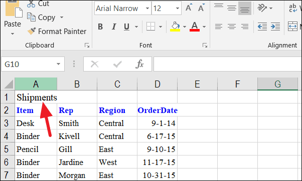
Merge Cells Without Losing Data
To keep all data intact while merging cells, you can use Excel functions like the Ampersand (&) operator or the CONCAT function. These methods combine the contents of multiple cells into one without discarding any information.
Using the Ampersand Operator
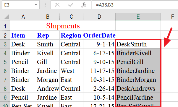
A3 and B3, type:=A3&B3This formula concatenates the contents of A3 and B3 directly.
=A3&" "&B3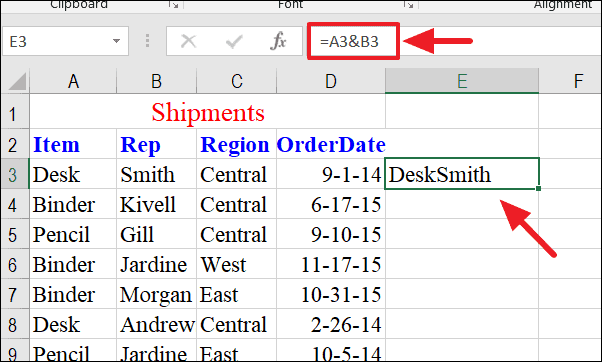
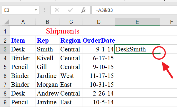
The formula adjusts automatically, combining the corresponding cells in each row.
If you’re merging cells that include dates, Excel might display unexpected numbers because it stores dates as serial numbers. To display the date properly, incorporate the TEXT function:
=A3&" - "&TEXT(D3,"dd mmm yyyy")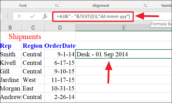
You can also add custom text within the formula. For example:
=A3&" in "&B3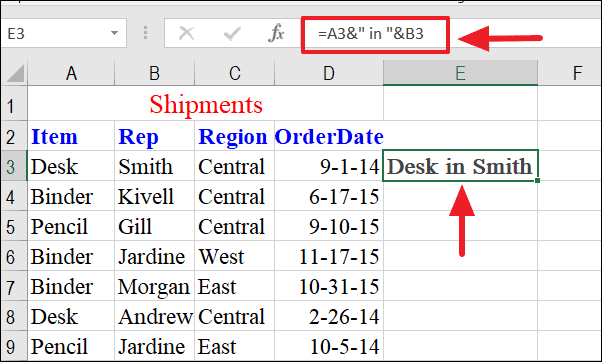
Using the CONCAT Function
The CONCAT function, or CONCATENATE in earlier Excel versions, is another way to merge cell contents without losing data.
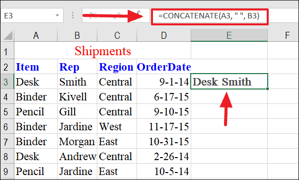
=CONCAT(A3,B3)=CONCAT(A3," ",B3)This adds a space between the merged data.
=CONCAT(A3," in ",B3)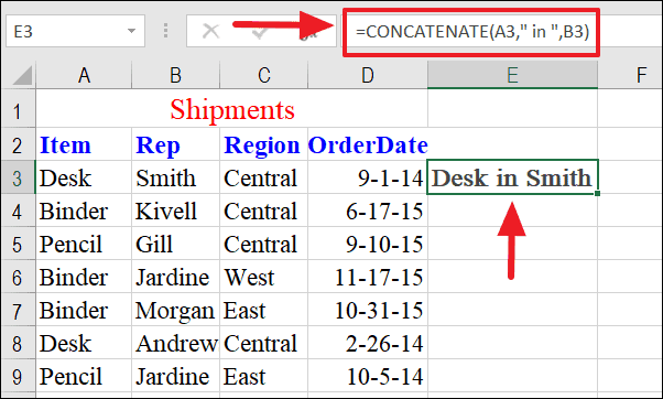
When merging cells that include dates, use the TEXT function to format the date correctly:
=CONCAT(A3," ",TEXT(D3,"dd mmm yyyy"))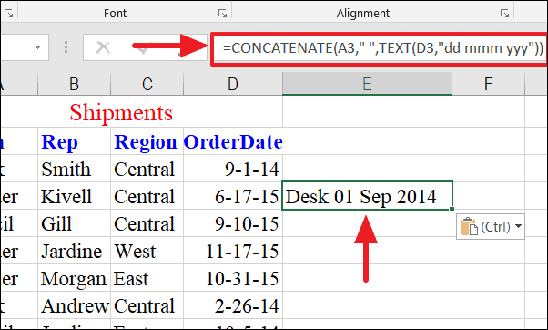
Using the Merge & Center Feature
Excel’s Merge & Center feature allows you to combine multiple cells into one larger cell, which is useful for formatting headers or titles across several columns.
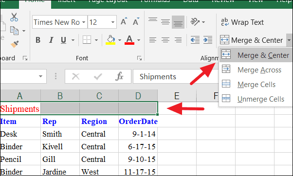
This combines the selected cells into one and centers the content.
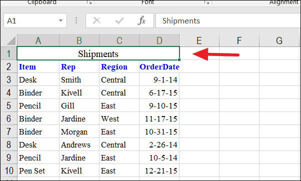
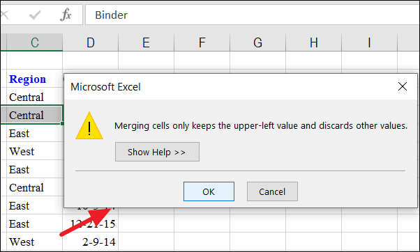
Note: When using this feature, only the data in the upper-left cell is retained. Excel will warn you if data from other cells will be lost.
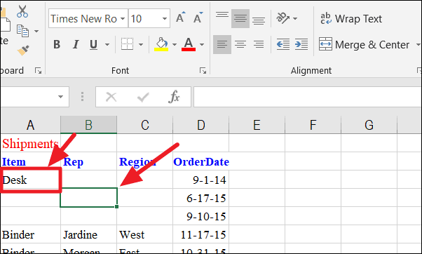
Unmerging Cells
To split merged cells back to their original state:
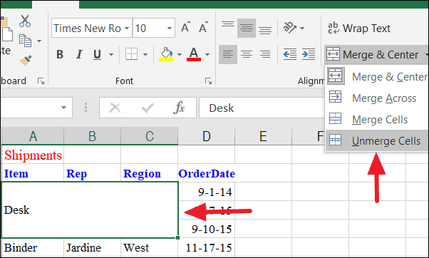
The cell will revert to individual cells, but only the content from the original upper-left cell remains.
Utilizing these techniques allows you to merge and combine cells in Excel effectively, ensuring that all your important data is preserved and your spreadsheets remain organized.


