
Multiplication is a fundamental operation in Excel, essential for data analysis and computations. Whether you’re multiplying numbers, cells, or entire ranges, Excel offers several methods to accomplish this efficiently.
Using the PRODUCT function to multiply in Excel
The PRODUCT function in Excel simplifies the process of multiplying multiple numbers, cells, or ranges. This function is particularly useful when dealing with large arrays of data, as it allows you to multiply a series of numbers without entering each one individually.
Enter. The formula should look like =PRODUCT(B1:B5), and the cell will display the product of the selected numbers.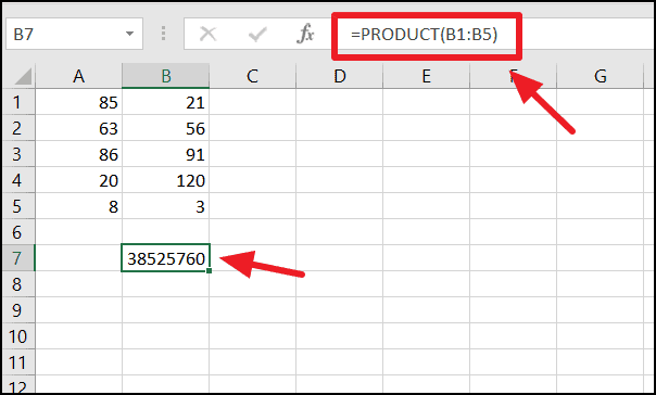
Multiplying in Excel using the multiplication operator
Another common way to perform multiplication in Excel is by using the multiplication operator, the asterisk (*). This method is straightforward and allows you to multiply numbers, individual cells, or ranges directly in a formula.
Multiplying numbers directly
=), followed by the numbers you want to multiply, separated by the multiplication operator. For example, =5*10.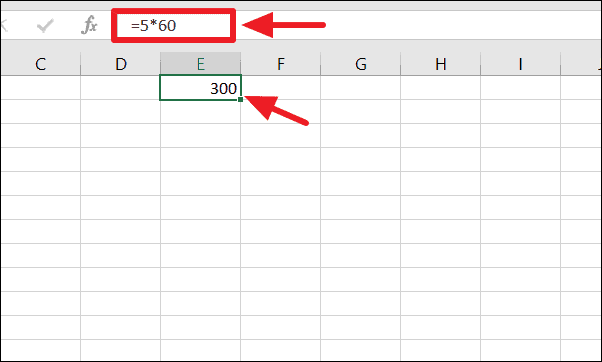
Multiplying cells
You can multiply the values of cells by referencing them in your formula.
=) followed by the cell references separated by the multiplication operator. For example, to multiply the values in cells A1 and B1, enter =A1*B1.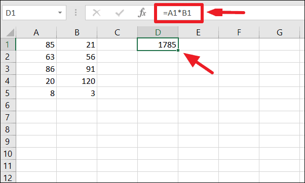
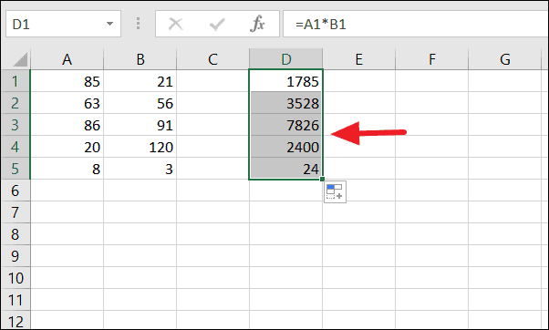
Multiplying columns of numbers
To multiply two columns of numbers, you can use the same multiplication formula and then copy it down the column.
=A1*B1.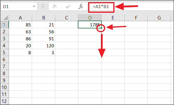
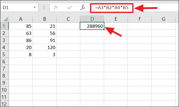
Multiplying multiple cells individually
To multiply several specific cells together, you can include each cell reference in your formula, separated by the multiplication operator.
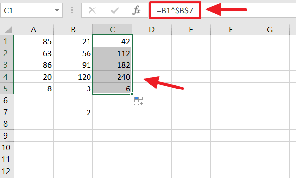
Multiplying a column by a fixed number
If you need to multiply an entire column of numbers by a constant value, you can use an absolute cell reference to lock the cell containing the constant.
=B1*$B$7, where $B$7 locks the reference to cell B7.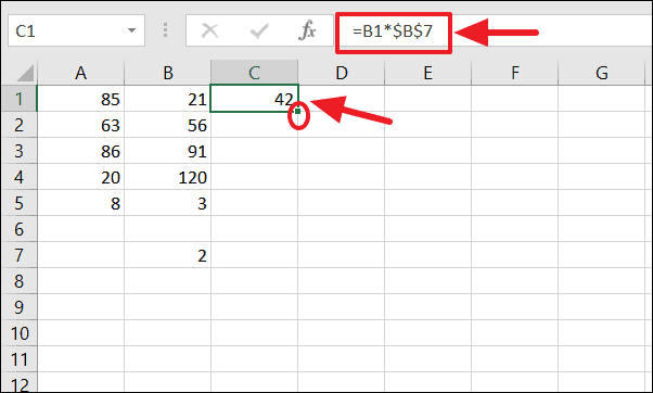
If using absolute cell references seems complicated, you can achieve the same result using the Paste Special feature to multiply a column by a constant number without writing a formula.
Copy or pressing Ctrl + C.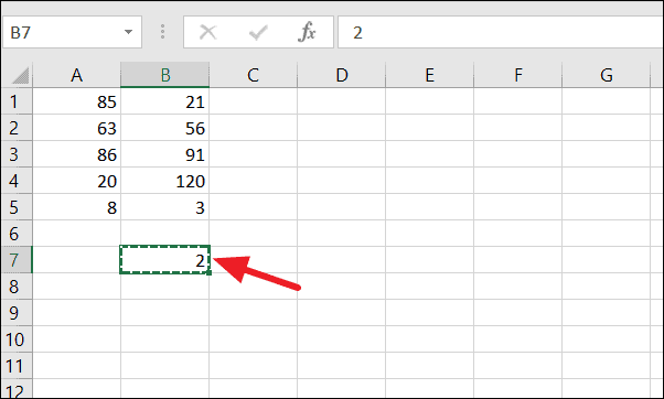
Paste Special.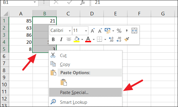
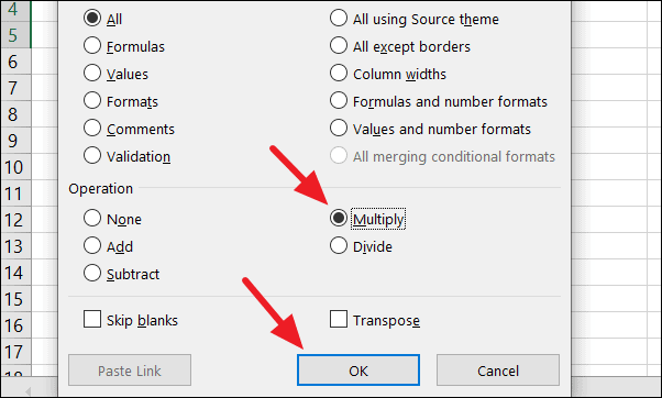
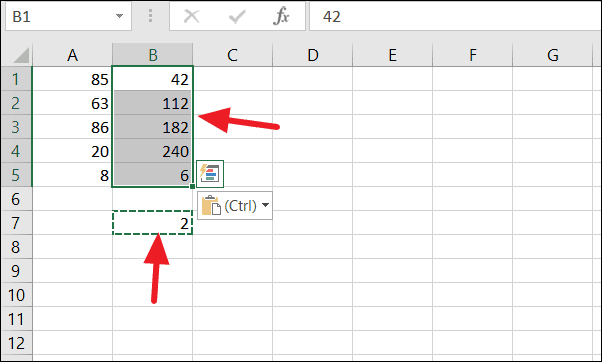
Excel will multiply each selected cell by the constant number, replacing the original values with the results.
By mastering these methods, you can efficiently perform multiplication tasks in Excel, enhancing your data analysis and spreadsheet calculations.


