How to Subtract in Excel

Excel is an invaluable tool for performing arithmetic operations, and subtraction is one of the fundamental calculations you can execute effortlessly. Understanding how to subtract numbers in Excel can enhance your data analysis and computational efficiency.

Subtracting Between Cells

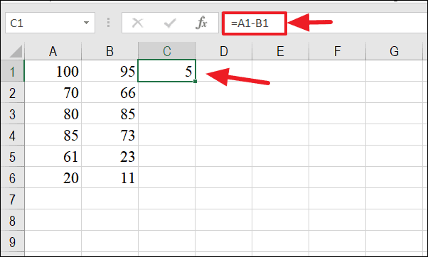
To subtract the value in one cell from another, use the cell references with the minus (-) operator. Begin your formula with an equal sign (=) followed by the cell references separated by the minus sign.

=Cell1 - Cell2

For instance, in the example below, cell C1 contains a formula that subtracts the value in cell B2 from the value in cell A1.

Subtracting Columns in Excel

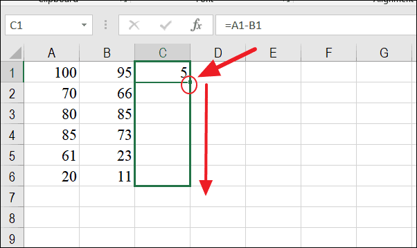
To apply subtraction across an entire column, enter the subtraction formula in the first cell, and then copy it to the remaining cells in the column. Click on the cell containing the formula, hover over the bottom-right corner until the fill handle (a small green square) appears, and drag it down over the cells you wish to populate.

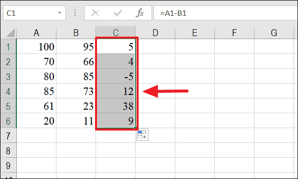
The subtraction formula is now extended to the entire range, and the results are displayed accordingly in column C.

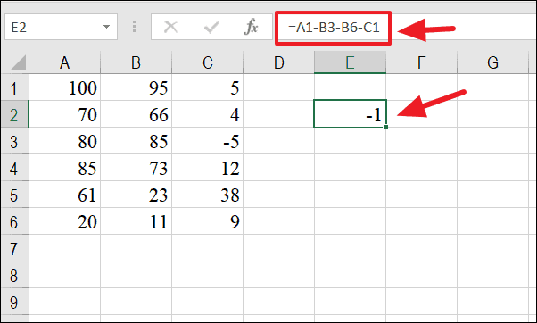
To subtract multiple cells individually, you can adjust the formula to include additional cell references separated by the minus sign.

Subtracting Numbers in a Cell

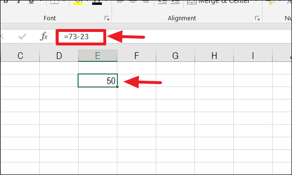
You can perform subtraction directly within a single cell by typing the numbers separated by the minus sign. Start the formula with an equal sign (=) to let Excel know you're entering a formula.

=Number1 - Number2

For example, entering =73 - 23 in cell E2 and pressing Enter will display the result, which is 50.

Subtracting Multiple Cells Using the SUM Function

When you need to subtract the sum of several cells from another value, the SUM function can simplify your formula. By wrapping the cells you want to sum within the SUM function and adding a minus sign before it, you can subtract the total from your initial value.

For example, to subtract the sum of cells A2 through A6 from cell A1, use the following formula:

=A1 - SUM(A2:A6)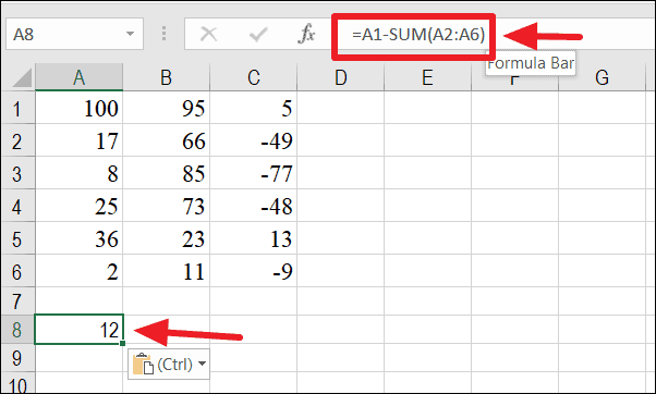

Subtracting the Same Number from a Column of Numbers

If you need to subtract the same number from a range of cells, you can utilize an absolute cell reference to lock the reference to that specific cell. This is done by placing a dollar sign ($) before the column letter and row number in the cell reference.

For example, to subtract the value in cell B8 from cells B1 through B6, you would create an absolute reference to B8 like this: $B$8. Your formula would look like:

=B1 - $B$8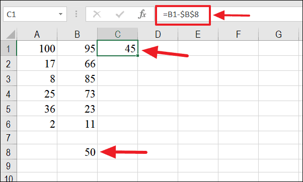

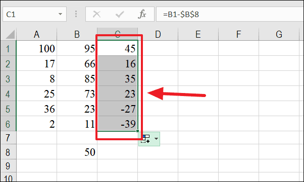
After entering the formula in the first cell, use the fill handle to drag the formula down to the other cells in the column. This action applies the same subtraction operation to each cell while keeping the reference to $B$8 constant.

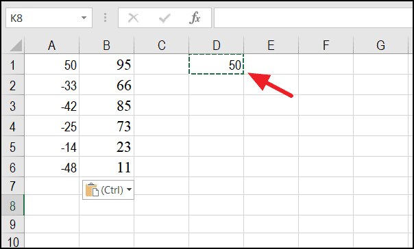
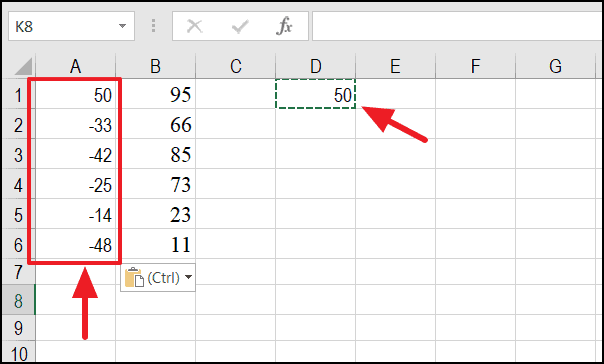
An alternative method is to subtract the number without using a formula by employing the Paste Special feature. Copy the cell containing the number you want to subtract (e.g., cell D1), select the range of cells from which you want to subtract the number (A1:A6), right-click, and choose Paste Special.