When names are combined into a single column in Excel, it can make data management tasks like sorting and filtering more challenging. Separating first names, middle names, and last names into individual columns enhances the utility and efficiency of your data.
Separate Names in Excel Using Flash Fill
Flash Fill is a powerful feature in Excel 2013 and later versions that automatically fills your data when it senses a pattern. It’s an efficient way to split names without complex formulas or manual copying.
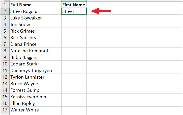
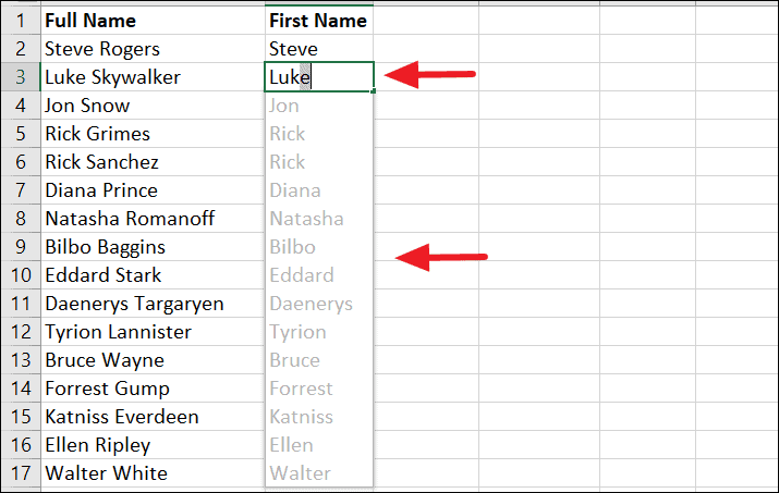
Enter key to accept the suggestions. Excel will automatically fill the column with the first names extracted from the full names.
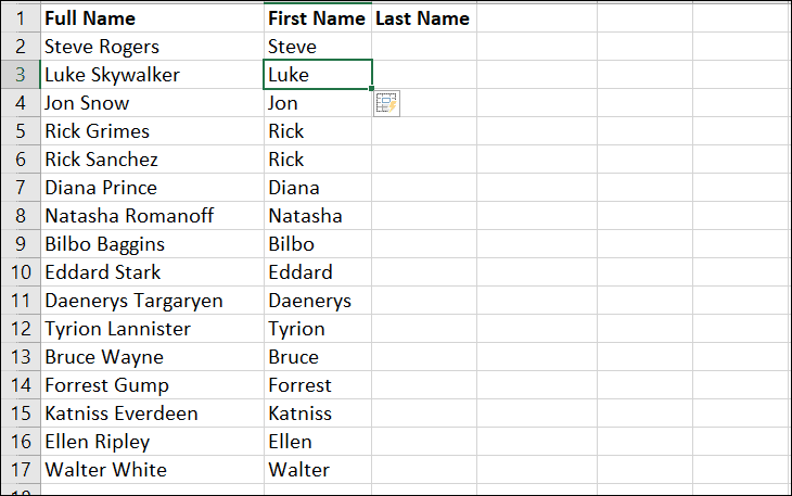
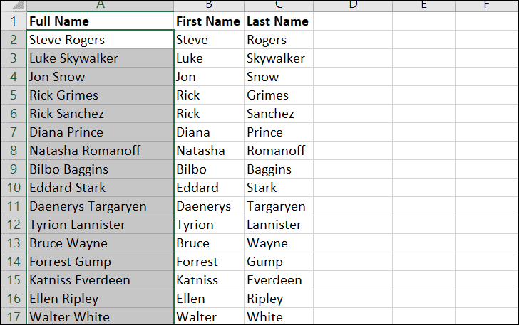
The result will be your first and last names separated into different columns:

If Flash Fill doesn’t automatically suggest the fill, you can trigger it manually. After typing the example(s), select the cells where you want the data filled. Then, go to the Data tab and click on the Flash Fill button in the Data Tools group.
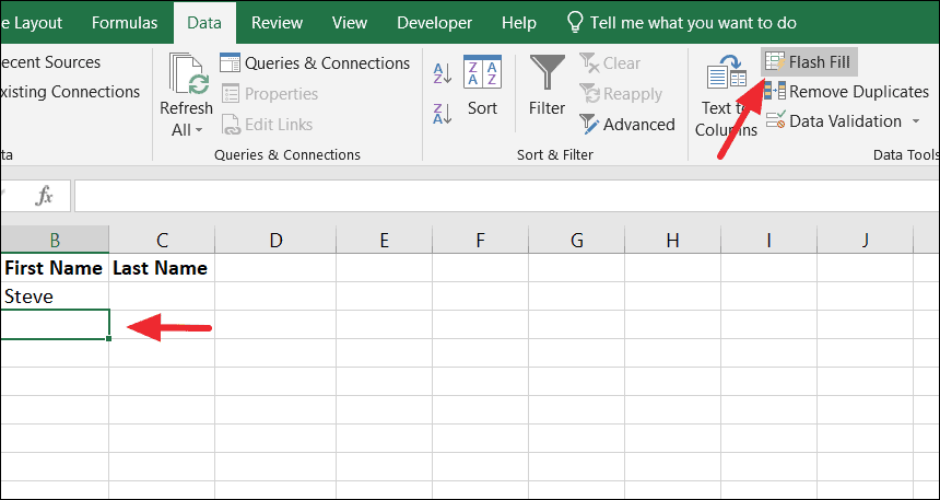
Alternatively, you can press Ctrl + E to activate Flash Fill. Excel will populate the cells based on the recognized pattern.
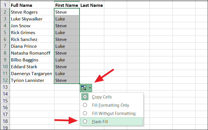
If Excel doesn’t detect the pattern after the first entry, you can help it by providing more examples. Type the desired output in the next few cells, then use the fill handle to drag down. Click on the Auto Fill Options icon that appears, and select Flash Fill from the dropdown menu to populate the rest.
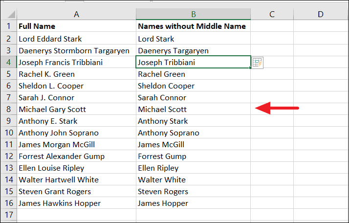
Extract Middle Names Using Flash Fill
Flash Fill can also be used to extract middle names or remove them from full names.
Enter to accept the suggestions.To remove middle names from full names, type the first and last name without the middle name in the adjacent cell. Provide a couple of examples, and Flash Fill will recognize the pattern to remove middle names from the rest of the entries.
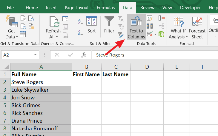
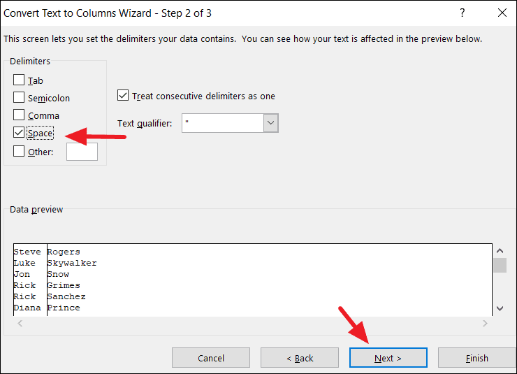
Separate Names Using Text to Columns Wizard
The Text to Columns feature in Excel allows you to split data from one column into multiple columns based on a delimiter such as a space or comma.
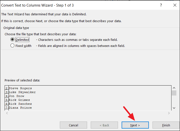
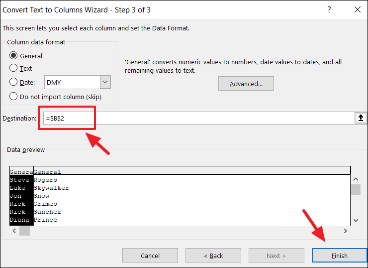
The full names will be split into separate columns based on the delimiter.
Note: This method creates static data. If the original names change, you will need to repeat the process to update the separated names.
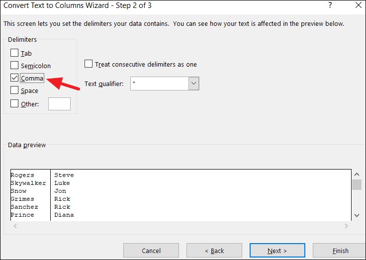
Split Names Separated by Commas
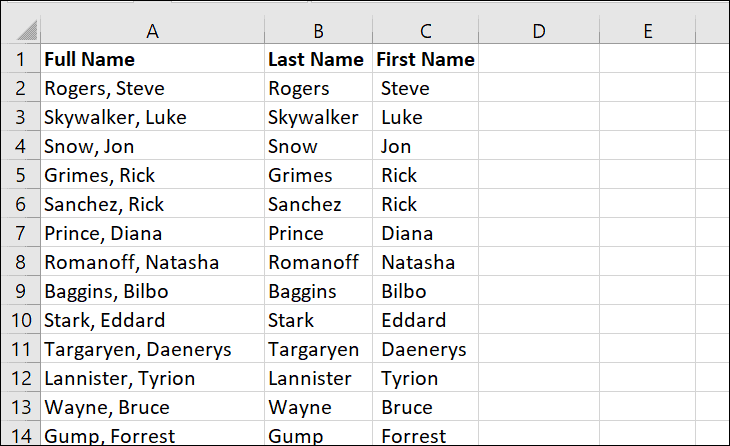
If your names are formatted with commas, such as “Doe, John”, you can still use the Text to Columns feature to separate them.
Separate Names Using Formulas
Using formulas to separate names provides dynamic results that update automatically when the original data changes. This method is flexible but requires a bit more effort to set up.
Extract First and Last Names Using Formulas
Get the First Name
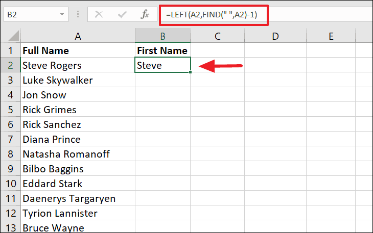
To extract the first name from a full name in cell A2, use the following formula:
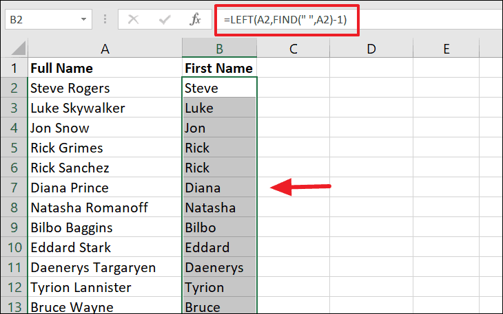
=LEFT(A2,FIND(" ",A2)-1)This formula finds the position of the space character and extracts all characters to the left of it.
Copy this formula down the column to extract first names from other full names.
Get the Last Name
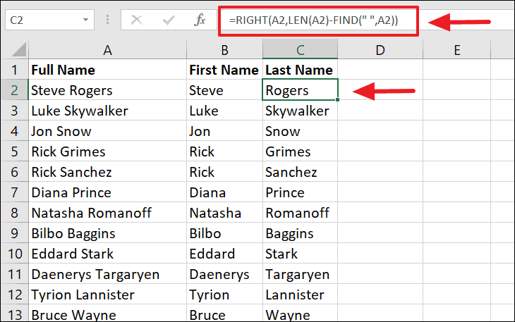
To extract the last name, use this formula:
=RIGHT(A2,LEN(A2)-FIND(" ",A2))This formula calculates the number of characters after the space and extracts them from the right.
Extract First, Middle, and Last Names Using Formulas
For names that include a middle name or initial, you can adjust the formulas to account for additional spaces.
Get the First Name
The formula for the first name remains the same:
=LEFT(A2,FIND(" ",A2)-1)Get the Middle Name
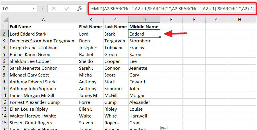
To extract the middle name, use the following formula:
=MID(A2,FIND(" ",A2)+1,FIND(" ",A2,FIND(" ",A2)+1)-FIND(" ",A2)-1)This formula locates the positions of the first and second spaces to isolate the middle name.
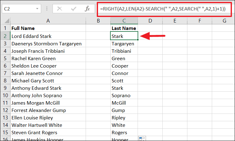
Get the Last Name
To get the last name when there’s a middle name, use this formula:
=RIGHT(A2,LEN(A2)-FIND(" ",A2,FIND(" ",A2)+1))This formula finds the position of the second space and extracts the text after it.
By utilizing these methods, you can efficiently separate names in Excel, improving data organization and accessibility. Whether you prefer the automation of Flash Fill, the control of Text to Columns, or the dynamism of formulas, Excel offers powerful tools to handle your data effectively.


