How to Set Print Area in Google Sheets

Printing specific sections of a Google Sheets document requires careful setup to ensure only the necessary information appears on paper. Incorrectly configuring the print area can lead to unwanted data being printed, resulting in wasted resources.

In Google Sheets, the print area determines which parts of your spreadsheet will be included when you print, allowing you to focus on particular cell ranges rather than the entire sheet.

Unlike Excel, where you can set permanent print areas and layouts, Google Sheets requires you to adjust the print settings each time you print to customize the output. This flexibility lets you choose between printing the entire workbook, a single sheet, or selected cells.

This guide will walk you through various methods to set the print area in Google Sheets.

Setting the Print Area for Selected Cells

Imagine you have a contact list in Google Sheets with columns for names, addresses, and phone numbers. If you only need to print the list of names, you can set the print area to include only that specific column.

By default, Google Sheets prints all cells containing data. To print only a specific range of cells, follow these steps:

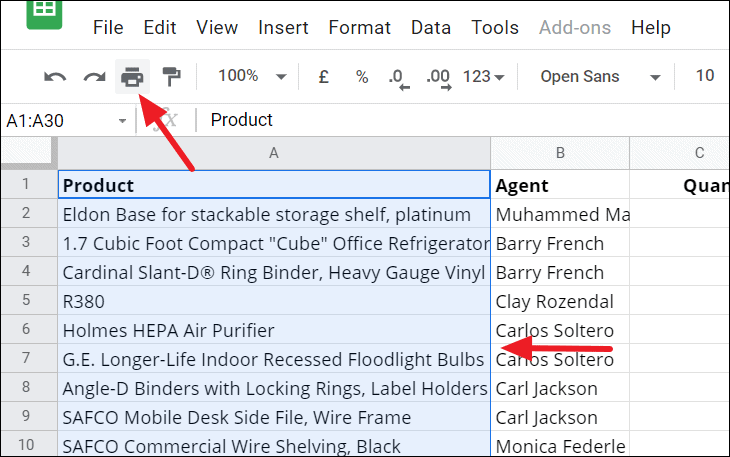
Open your spreadsheet and select the range of cells you wish to print. Ensure that the selected cells form a continuous range; otherwise, only the last selected range will be printed. For example, select cells A1 to A30 for the “Name” column.

Click on the printer icon in the toolbar or go to the File menu and select Print. You can also use the keyboard shortcut CTRL + P.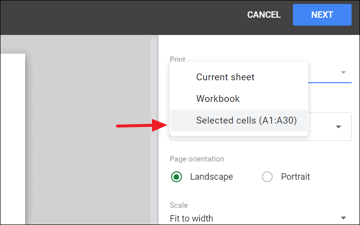

In the Print settings window, you’ll see a preview of your printout along with various options on the right. Click on the dropdown menu under “Print” and choose “Selected cells.” The preview will update to show only the cells you’ve selected.

Click Next to proceed to the printer settings and complete the printing process. Only your selected cells will be printed.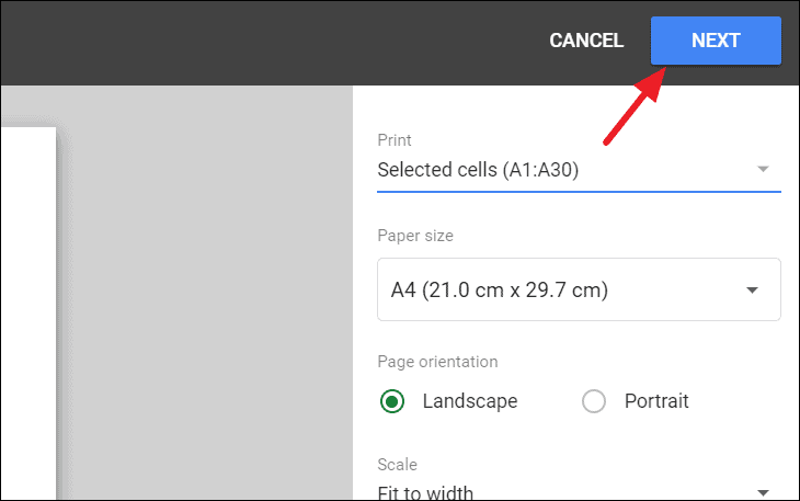

Printing the Current Sheet or Entire Workbook

By default, when you print in Google Sheets without selecting any cells, it prints the current sheet. To confirm or change this setting:

Open the spreadsheet you want to print. Click on the File menu and select Print or use the keyboard shortcut CTRL + P.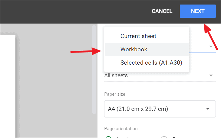

In the Print settings window, ensure that the dropdown menu under “Print” is set to “Current sheet.” This option will print all the data in the active worksheet.

If you wish to print the entire workbook, including all sheets, click on the dropdown menu under “Print” and select “Workbook.”

Click Next to proceed to the printer settings and print the entire workbook.

Customizing the Page Layout to Set the Print Area

You can further refine your print area by adjusting the page size, scale, and margins. These settings help control how much data appears on each page and how it is formatted.

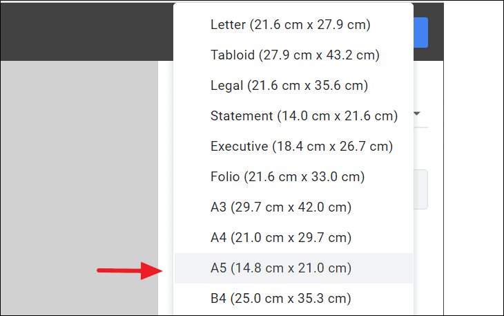
Adjusting Page Size

In the Print settings window, find the “Page size” dropdown menu.

Select the desired page size from the list. Choosing a smaller page size reduces the number of cells printed on each page, effectively limiting the print area.

Modifying Scale Settings

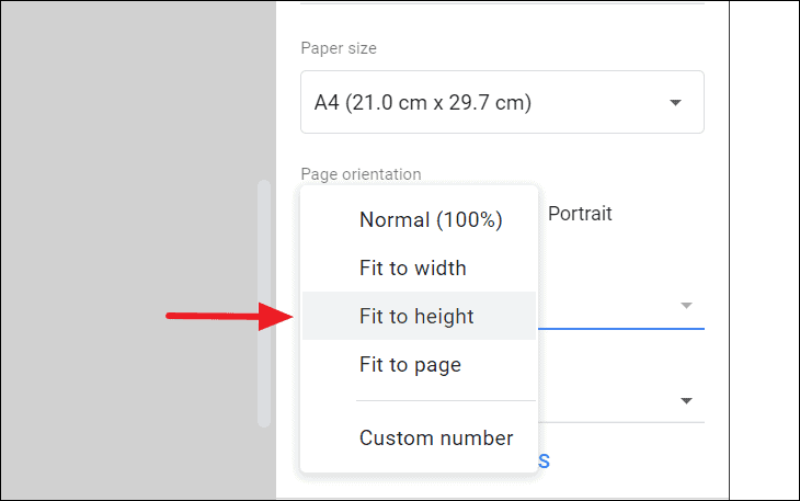
The scale setting adjusts how your data fits on the page:

Click on the “Scale” dropdown menu in the Print settings.

Choose one of the following options:

Normal – Maintains the default scaling.
Fit to Width – Fits all columns onto one page width-wise, ideal for sheets with many columns.
Fit to Height – Fits all rows onto one page height-wise, suitable for sheets with many rows.
Fit to Page – Fits all data onto a single page, best for small spreadsheets.

Setting Margins

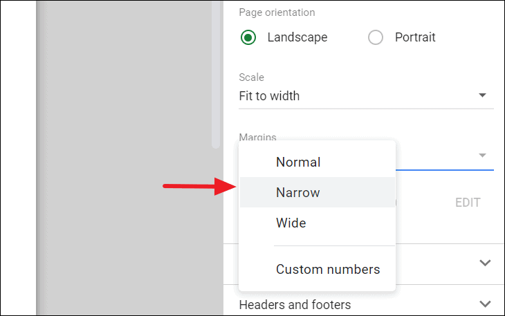
Margins affect the amount of white space around your data:

In the Print settings, click on the “Margins” dropdown menu.

Select one of the options:

Normal – Standard margin size.
Narrow – Reduces margins to allow more data per page.
Wide – Increases margins, resulting in more white space.

After adjusting these settings, click Next to proceed to the printer settings and finalize your print job.

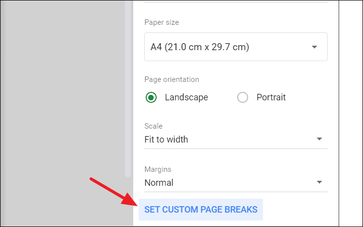
Setting the Print Area Using Custom Page Breaks

Custom page breaks allow you to specify exactly where a new page should start in your printed document. This is particularly useful for controlling how data is divided across pages.

In the Print settings window, click on SET CUSTOM PAGE BREAKS at the bottom.

You’ll see a preview of your sheet with blue lines indicating the current page breaks.

Click and drag the blue lines to adjust where pages break. For example, if you want only 25 rows per page instead of the default 30, move the horizontal page break line up to row 25.

After adjusting the page breaks, click CONFIRM BREAKS to save your changes.

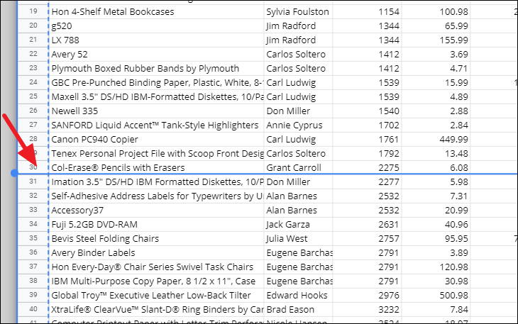
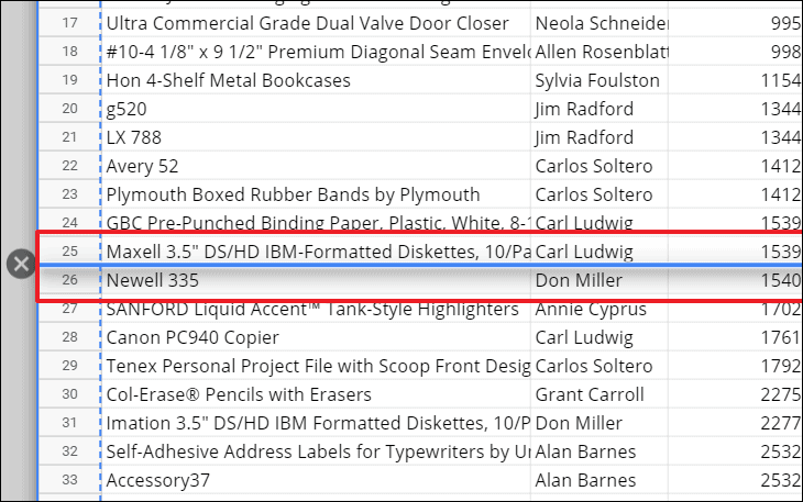
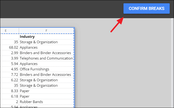
Proceed to print your document with the new page breaks in place.

Printing Header Rows on Each Page

Including header rows on every printed page helps to identify the data columns without having to refer back to the first page.

Open your spreadsheet and click on the View menu at the top.

Navigate to Freeze and select 1 row to freeze the top row, which typically contains your headers.

The frozen header row will now appear at the top of each printed page.

Click the printer icon or press CTRL + P to open the Print settings and preview your document.

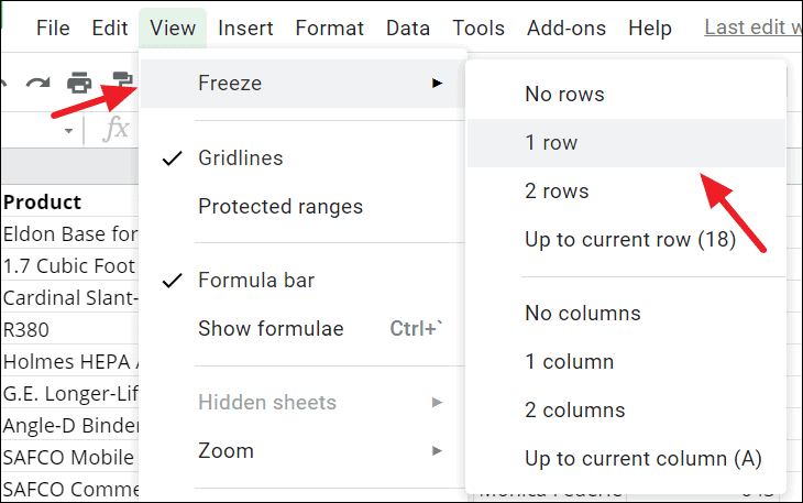
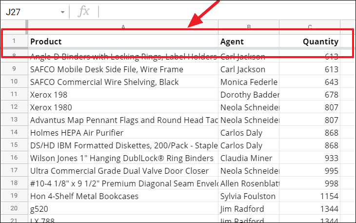
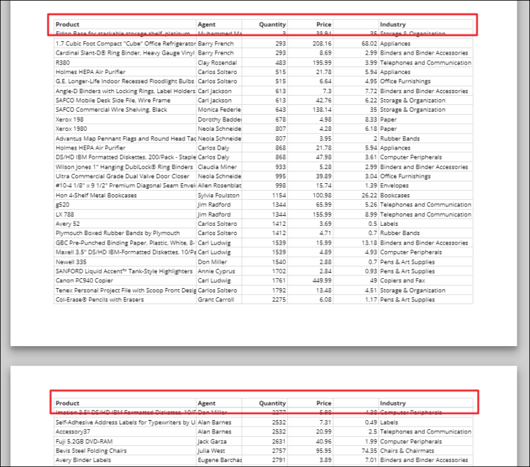
Proceed to print, and your header row will be included on each page.

By utilizing these methods, you can effectively control what parts of your Google Sheets document are printed, ensuring that only the necessary information is included in your printouts.