
Excel users often need to separate data within a cell into multiple cells for better organization and analysis. Splitting cells can simplify data handling, especially when working with extensive lists like full names that need to be divided into first and last names.
Split cells in Excel using Flash Fill feature
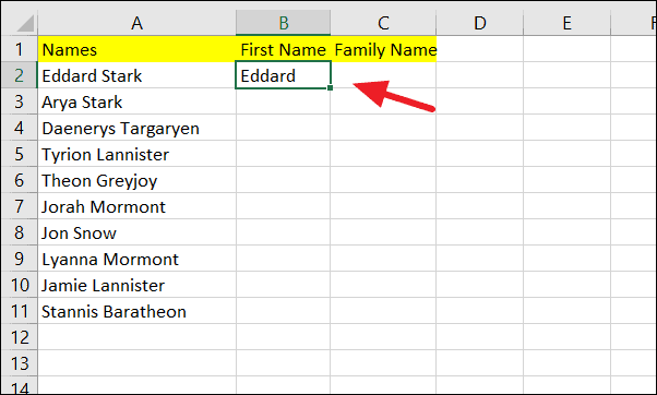
The Flash Fill feature in Excel is an efficient tool that recognizes patterns in your data and fills out the remaining entries based on the example you provide. It’s one of the quickest methods to split cells without complex formulas or data tools.
Data tab on the Excel ribbon. Click on the Flash Fill button in the Data Tools group.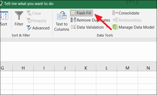
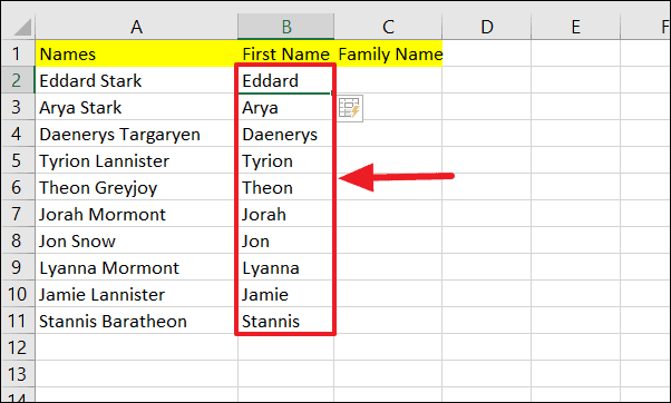
Ensure that the pattern is clear to Excel so it can accurately fill the remaining cells. Flash Fill works best when your data is consistent.
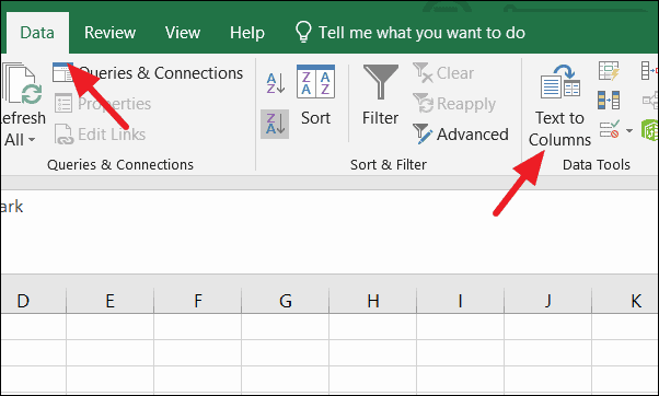
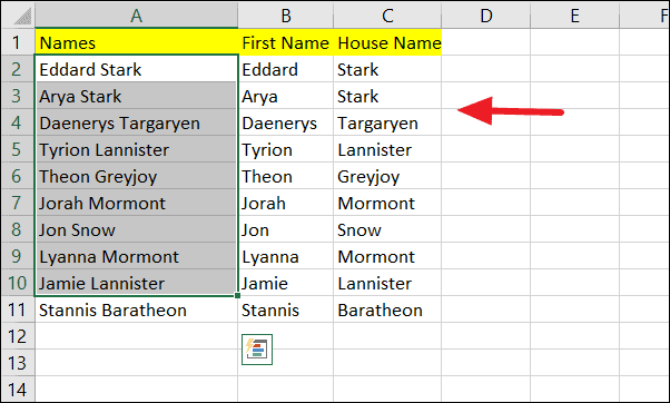
Split cells in Excel using Text to Columns feature
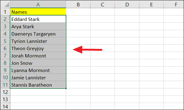
The Text to Columns tool allows you to split a single column of data into multiple columns based on delimiters such as spaces, commas, or other characters.
Delimited as the original data type since the names are separated by spaces. Click Next.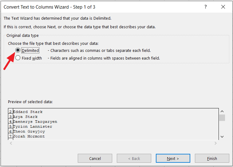
Space option and ensure other delimiters are unchecked. You can view how your data will be split in the Data preview section. Click Next.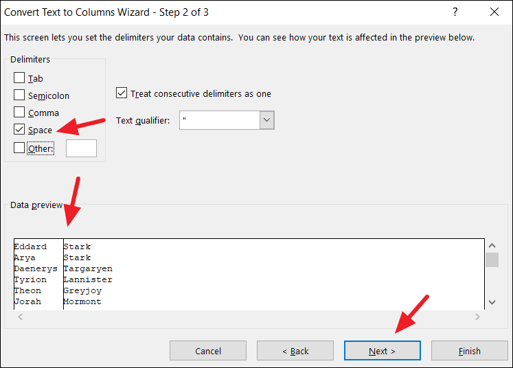
General. In the Destination field, specify where you want the split data to appear. By default, it will overwrite the original data, so it’s advisable to select a new location (e.g., starting at cell B2). Click Finish to apply the changes.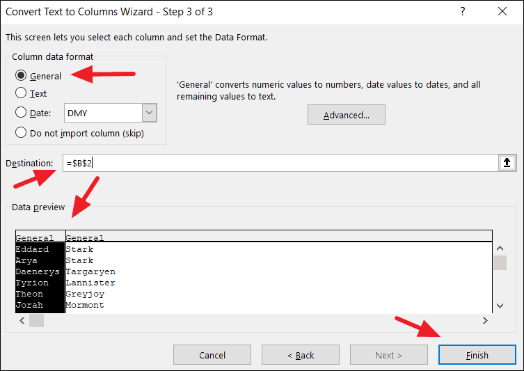
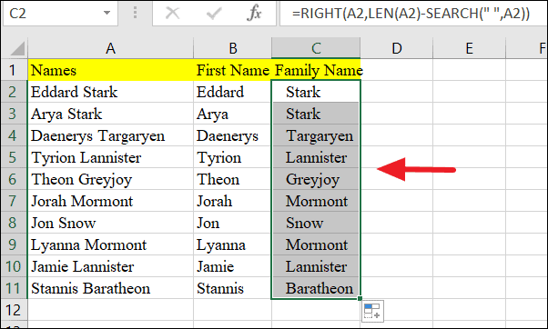
Split cells in Excel using formulas
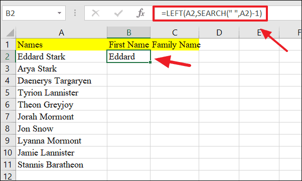
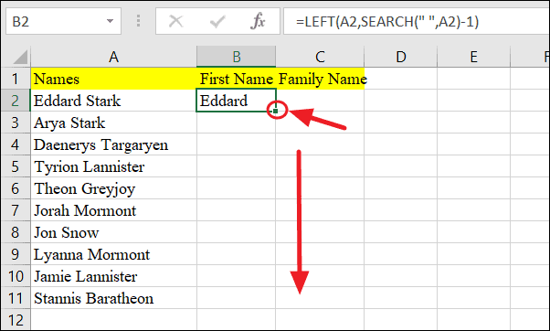
Formulas offer a dynamic way to split cells, with the advantage that they automatically update if the original data changes. This method involves using text functions to extract parts of a string.
=LEFT(A2,SEARCH(" ",A2)-1)This formula finds the position of the space character in the text and extracts all characters to the left of it.
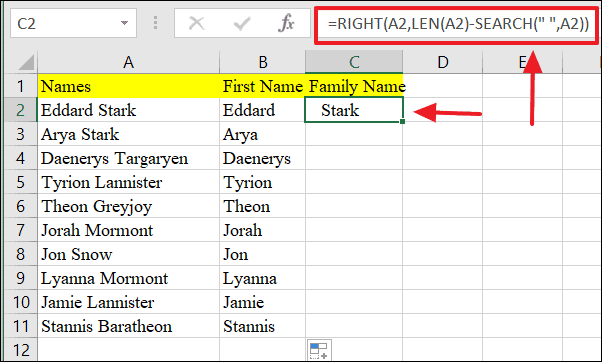
=RIGHT(A2,LEN(A2)-SEARCH(" ",A2))This formula calculates the length of the text, finds the position of the space character, and extracts the characters to the right of the space.
Splitting cells in Excel can greatly enhance your data management and analysis capabilities. Whether you prefer the simplicity of Flash Fill, the control of Text to Columns, or the dynamism of formulas, Excel offers flexible solutions to meet your data splitting needs.


