Adding up columns or rows of numbers is something most of us are required to do quite often. For example, if you store crucial data such as sales records or price lists in the cells of a single column, you may want to quickly know the total of that column. So it’s necessary to know how to sum a column in Excel.
There are several ways you can sum or total a column/row in Excel including, using a single click, the AutoSum feature, SUM function, filter feature, SUMIF function, and by converting a dataset into a table. In this article, we will see the different methods for adding up a column or row in Excel.
SUM a Column with One Click using Status Bar
The easiest and quickest way to calculate the total value of a column is to click on the letter of the column with the numbers and check the ‘Status’ bar at the bottom. Excel has a Status bar at the bottom of the Excel window, which displays various information about an Excel worksheet including average, count, and sum value of the selected cells.
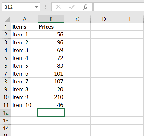
Let us assume you have a table of data as shown below and you want to find the total of the prices in column B.
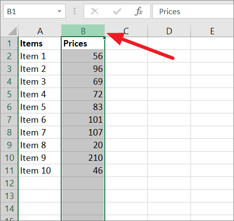
All you have to do is select the entire column with the numbers you want to sum (Column B) by clicking on the letter B at the top of the column and look at the Excel Status bar (next to the zoom control).
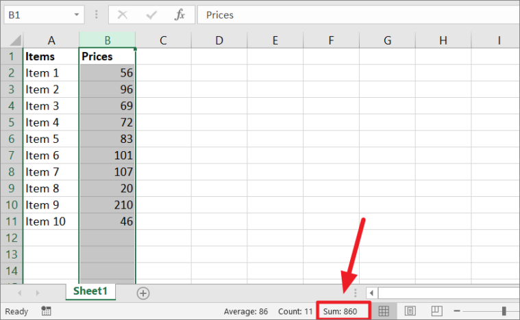
There you will see the total of the selected cells along with the average and count values.
You can also select data range B2 to B11 instead of the whole column and see the Status bar to know the total. You can also find the total of numbers in a row by selecting the row of values instead of a column.
The benefit of using this method is that it automatically ignores the cells with text values and only sums the numbers. As you can see above, when we selected the whole column B including cell B1 with a text title (Price), it only summed up the numbers in that column.
SUM a Column with AutoSum Function
Another quickest way to sum up a column in Excel is by using the AutoSum feature. AutoSum is a Microsoft Excel feature that allows you to quickly add up a range of cells (column or row) containing numbers/integers/decimals using the SUM function.
There is an ‘AutoSum’ command button on both the ‘Home’ and ‘Formula’ tab of the Excel ribbon that will insert the ‘SUM function’ in the selected cell when pressed.
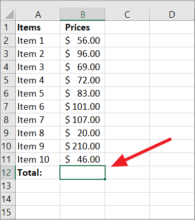
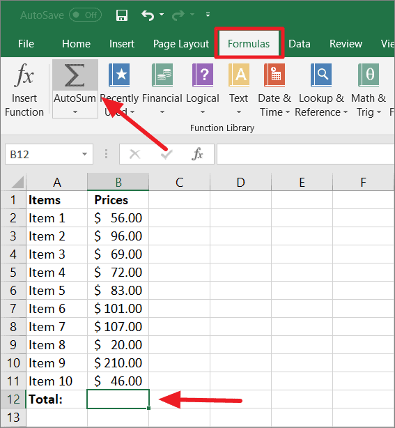
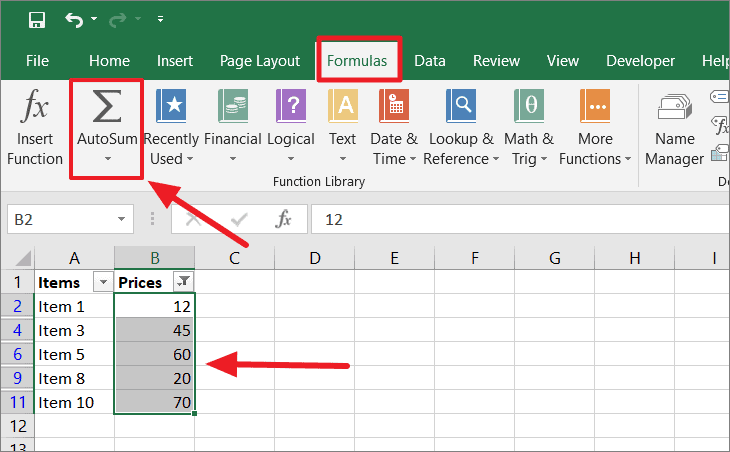
Suppose you have the table of data as shown below and you want to sum up the numbers in column B. Select an empty cell right below the column or the right end of a row of data (to sum a row) you need to sum.
Then, select the ‘Formula’ tab and click on the ‘AutoSum’ button in the Function Library group.
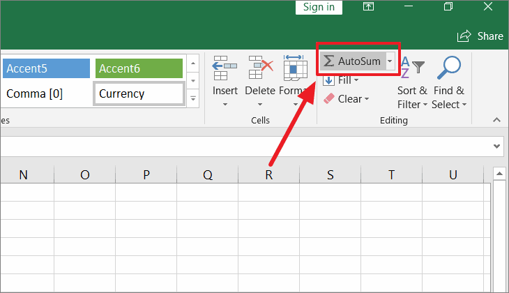
Or, go to the ‘Home’ tab and click on the ‘AutoSum’ button in the Editing group.
Either way, once you click the button, Excel will automatically insert the ‘=SUM()’ in the selected cell and highlights the range with your numbers (marching ants around the range). Check to see if the selected range is correct and if it’s not the correct range, you can change it by selecting another range. And the parameters of the function will auto-adjust according to that.
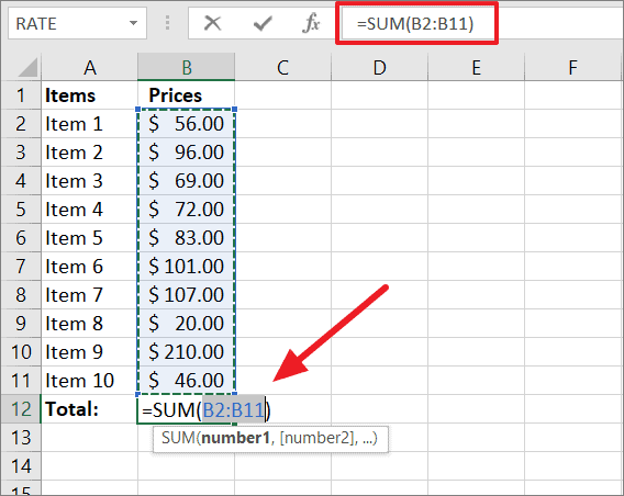
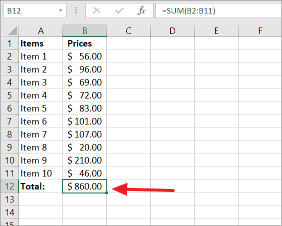
Then, just press Enter on your keyboard to see the sum of the entire column in the selected cell.
You can also invoke the AutoSum function using a keyboard shortcut.
To do that, select the cell, which is just below the last cell in the column for which you want the total, and use the below shortcut:
Alt+= (Press and hold the Alt key and press the equal sign = keyAnd it will automatically insert the SUM function and select the range for it. Then press Enter to total the column.
AutoSum lets you quickly sum a column or row with a single click or press of a keyboard shortcut.
However, there is a certain limitation to the AutoSum function, it would not detect and select the correct range in case there are any empty cells in the range or any cell that has a text value.
As you can see in the above example, cell B6 is empty. And when we entered the AutoSum function in cell B12, it only selects 5 cells above. It’s because the function perceives that cell B7 is the end of the data and returns only 5 cells for the total.
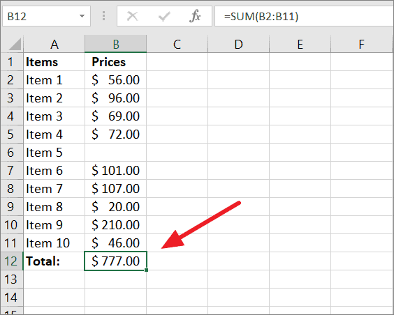
To fix this, you need to change the range by clicking-and-dragging with the mouse or type the correct cell references manually to highlight the whole column and press Enter. And, you will get the right result.
To avoid this, you can also enter the SUM function manually to calculate the sum.
SUM a Column by Entering the SUM Function Manually
Although the AutoSum command is quick and easy to use, sometimes, you may need to enter the SUM function manually to calculate the sum of a column or row in Excel. Especially, if you only want to add up some of the cells in your column or if your column contains any blanks cells or cells with a text value.
Also, if you want to show your sum value in any of the cells in the worksheet other than the cell right below the column or the cell after the row of numbers, you can use the SUM function. With the SUM function, you can calculate the sum or total of cells anywhere in the worksheet.
The Syntax of SUM Function:
=SUM(number1, [number2],...).number1(required) is the first numeric value to be added.number 2(optional) is the second additional numeric value to be added.
While number 1 is the required argument, you can sum up to a maximum of 255 additional arguments. The arguments can be the numbers you want to add up or cell references to the numbers.
Another benefit of using the SUM function manually is that you add up numbers in non-adjacent cells of a column or row as well as multiple columns or rows. Here’s how you use the SUM function manually:
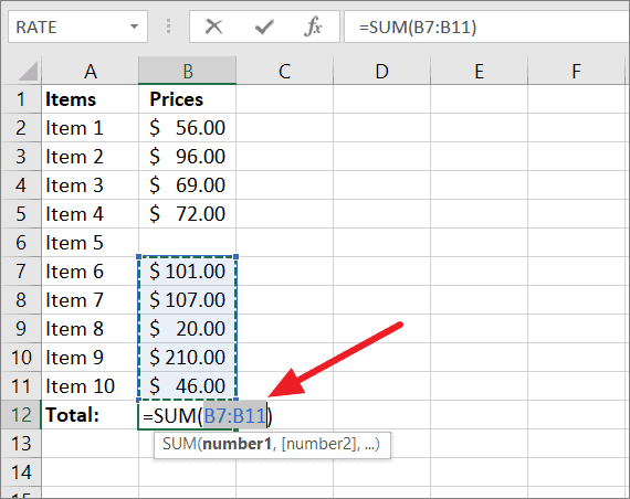
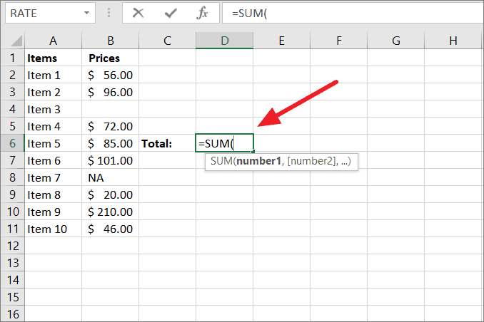
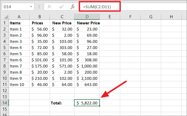
First, select the cell where you want to see the total of a column or row anywhere on the worksheet. Next, start your formula by typing =SUM( in the cell.
Then, select the range of cells with the numbers you want to sum or type the cell references for the range you want to sum in the formula.
You can either click-and-drag with the mouse or hold the shift key and then use the arrow keys to select a range of cells. If you want to enter cell reference manually, then type the cell reference of the first cell of the range, followed by a colon, followed by the cell reference of the last cell of the range.
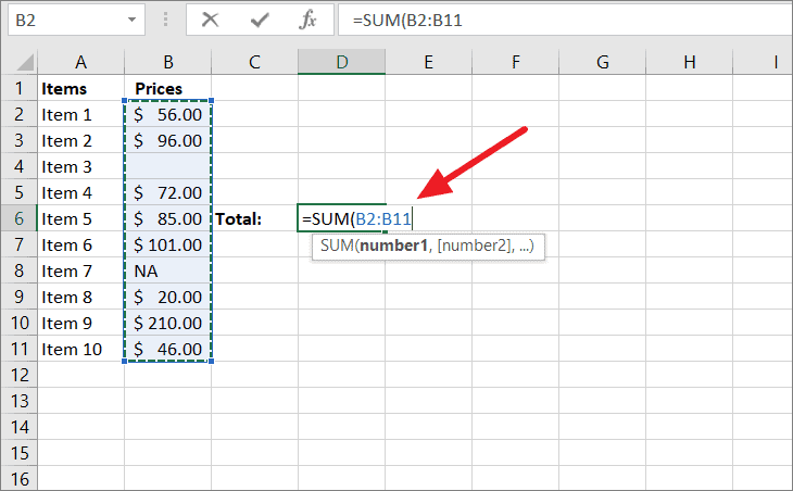
After you entered the arguments, close the bracket and press the Enter key to get the result.
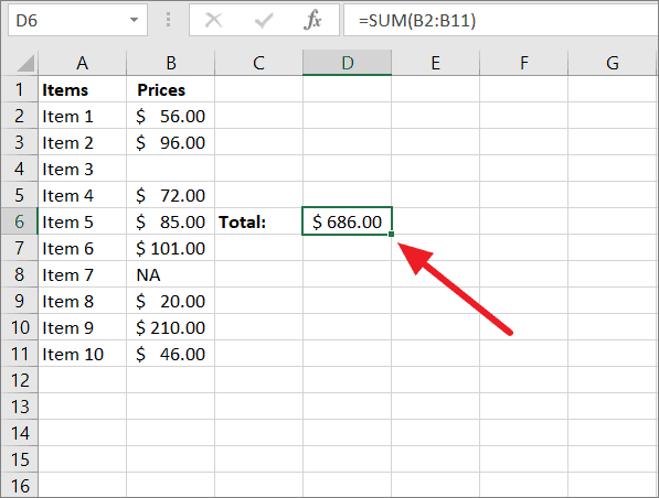
As you can see, even though the column has an empty cell and a text value, the function gives you the sum of all the selected cells.
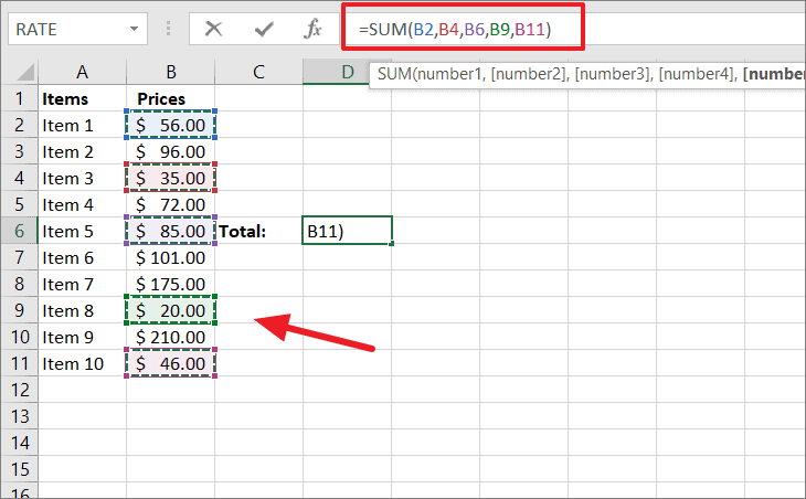
Summing Non-Continous Cells in a Column
Instead of summing up a range of continuous cells, you can also sum up non-continuous cells in a column. To select non-adjacent cells, hold the Ctrl key and click the cells you want to add up or type cell references manually and separate them with comms (,) in the formula.
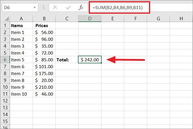
This will display the sum of only the selected cells in the column.
Summing Multiple Columns
If you want the sum of multiple columns, select multiple columns with the mouse or enter the cell reference of the first in the range, followed by a colon, followed by the last cell reference of the range for the arguments of the function.
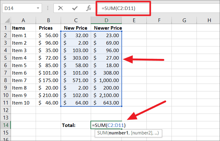
After you entered the arguments, close the bracket and press the Enter key to see the result.
Summing Non-Adjacent Columns
You can also sum non-adjacent columns using the SUM function. Here’s how:
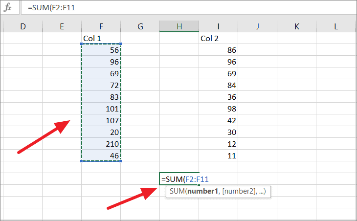
Select any cell in the worksheet where you want to show the total of the non-adjacent columns. Then, start the formula by typing the function =SUM( in that cell. Next, select the first column range with the mouse or type the range reference manually.
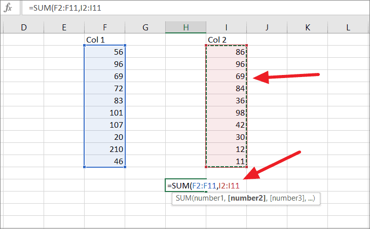
Then, add a comma and select the next range or type the second range reference. You can add as many ranges as you want in this way and separate each of them with a comma (,).
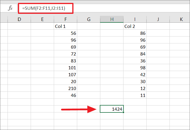
After the arguments, close the bracket, and press Enter to get the result.
Summing Column using Named Range
If you have a large worksheet of data and you want to quickly calculate the total of numbers in a column, you can use named ranges in the SUM function to find the total. When you create Named Ranges, you can use these names instead of the cell references which makes it easy to refer to data sets in Excel. It is easy to use named range in the function instead of scrolling down hundreds of rows to select the range.
Another good thing about using Named range is that you can refer to a data set (range) in another worksheet in the SUM argument and get the sum value in the current worksheet.
To use a named range in a formula, first, you need to create one. Here’s how you create and use a named range in the SUM function.
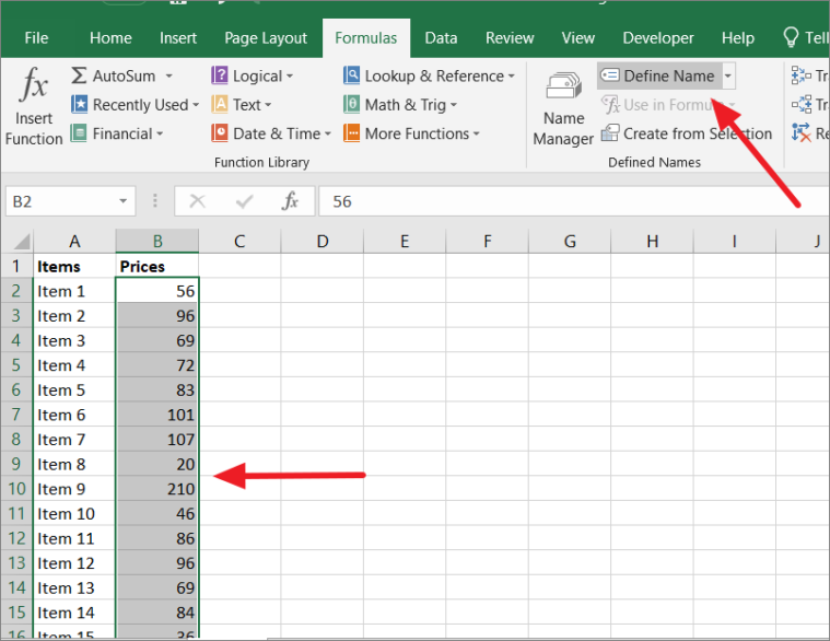
First, select the range of cells (without headers) for which you want to create a Named Range. Then, head to the ‘Formulas’ tab and click on the ‘Define Name’ button in the Defined Names group.
In the New Name dialogue box, specify the name you want to give to the selected range in the ‘Name:’ field. In the ‘Scope:’ field, you can change the scope of the named range as the whole Workbook or a specific worksheet. The scope specifies whether the named range would be available to the entire workbook or only a specific sheet. Then, click the ‘OK’ button.
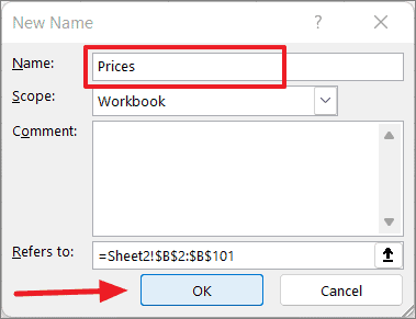
You can also change the reference of the range in the ‘Refers to’ field.
Alternatively, you can also name a range by using the ‘Name’ box. To do this, select the range, go to the ‘Name’ box on the left of the Formula bar (just above the letter A) and enter the name you wish to assign to the selected date range. Then, press Enter.
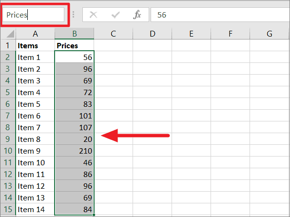
But when you create a named range using the Name box, it automatically sets the scope of the named range to the whole workbook.
Now, you can use the named range you created to quickly find the sum value.
To do this, select any empty cell anywhere on the workbook where you want to display the Sum result. And the type the SUM formula with the named range as is its arguments and press Enter:
=SUM(Prices)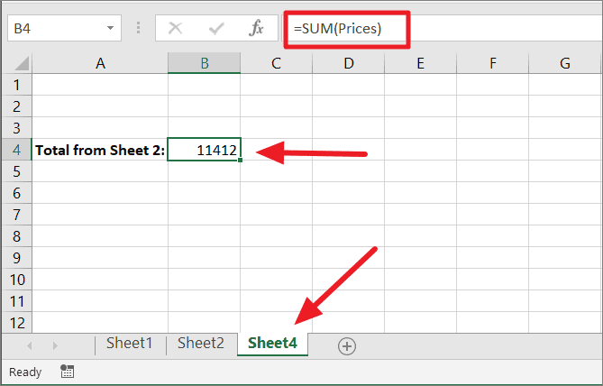
In the above example, the formula in Sheet 4 refers to the column named ‘Prices’ in Sheet 2 to get the sum of a column.
Sum Only the Visible Cells in a Column Using SUBTOTAL Function
If you have filtered cells or hidden cells in a data set or column, using the SUM function to total a column is not ideal. Because the SUM function includes filtered or hidden cells in its calculation.
The below example shows what happens when you sum a column with hidden or filtered rows:
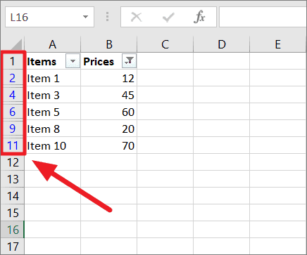
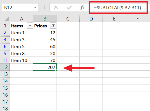
In the above table, we have filtered column B by prices that are less than 100. As a result, we have some filtered rows. You can notice that there are filtered/hidden rows in the table by the missing row numbers.
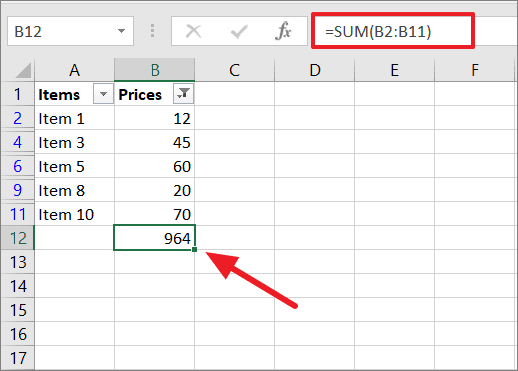
Now, when you sum the visible cells in column B using the SUM function, you should be getting ‘207’ as the sum value but instead, it shows ‘964’. Its because the SUM function also takes the filtered cells into account when calculating the sum.
This is why you cannot use the SUM function when filtered or hidden cells are involved.
If you don’t want the filtered/hidden cells to be included in the calculation when totaling a column and you only want to sum the visible cells, then you need to use the SUBTOTAL function.
SUBTOTAL Function
The SUBTOTAL is a powerful built-in function in Excel that allows you to perform various calculations (SUM, AVERAGE, COUNT, MIN, VARIANCE, and others) on a range of data and returns a total or an aggregate result of the column. This function only summarizes data in the visible cells while ignoring filtered or hidden rows. SUBTOTAL is a versatile function that can perform 11 different functions in visible cells of a column.
The Syntax of SUBTOTAL function:
=SUBTOTAL (function_num, ref1, [ref2], ...)Arguments:
function_num(required) – It is a function number that specifies which function to use for calculating the total. This argument can take any value from 1 to 11 or 101 to 111. Here, we need to sum the visible cells while ignoring filtered-out cells. For that, we need to use ‘9’.ref1(required) – The first named range or reference that you want to subtotal.ref2(optional) – The second named range or reference that you want to subtotal. After the first reference, you can add up to 254 additional references.
Summing a Column using SUBTOTAL Function
If you want to sum visible cells and exclude filtered or hidden cells, then follow these steps to use the SUBTOTAL function to sum a column:
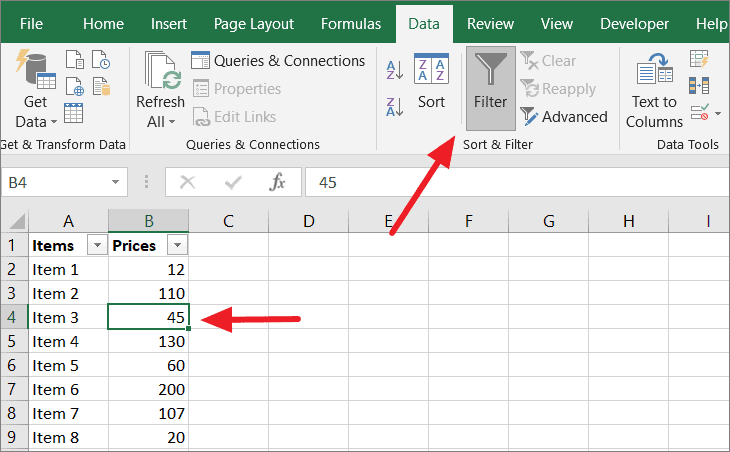
First, you need to filter your table. To do that, click on any cell within your data set. Then, navigate to the ‘Data’ tab and click the ‘Filter’ icon (funnel icon).
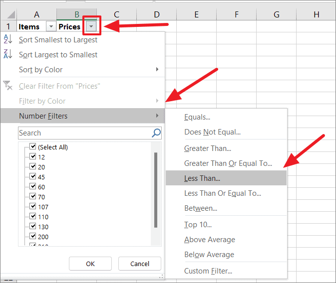
The arrows will appear next to column headers. Click on the arrow next to the column header with which you want to filter the table. Then, choose the filter option you wish to apply to your data. In the below example we want to filter column B with numbers less than 100.
In the Custom AutoFilter dialog box, we’re entering ‘100’ and clicking ‘OK’.
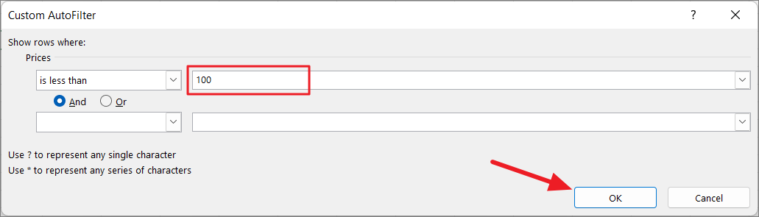
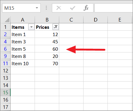
The numbers in the column are filtered by values less than 100.
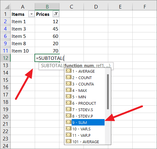
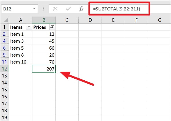
Now, select the cell where you wish to show the sum value and start typing the SUBTOTAL function. Once you open the SUBTOTAL function and type the bracket, you would see a list of functions you can use in the formula. Click ‘9 – SUM’ in the list or type ‘9’ manually as the first argument.
Then, select the range of cells you wish to sum or type the range reference manually and close the bracket. Then, press Enter.
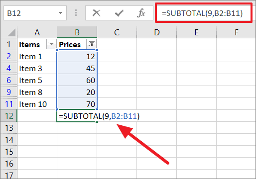
Now, you would get the sum (subtotal) of only the visible cells – ‘207’
Alternatively, you can also select the range (B2:B11) with the numbers that you wish to add up and click ‘AutoSum’ under the ‘Home’ or ‘Formulas’ tab.
It will automatically add the SUBTOTAL function at the end of the table and sums up the result.
Convert Your Data into an Excel Table to Get the Sum of Column
Another easy way that you can use to sum your column is by converting your spreadsheet data into an Excel table. By converting your data into a table, you can not only sum your column but can also perform many other functions or operations with your list.
If your data is not already in a table format, you need to convert it into an Excel table. Here’s how you convert your data into an Excel table:
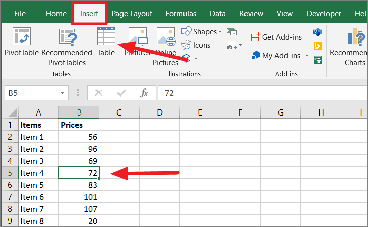
First, select any cell within the data set that you want to convert to an Excel Table. Then, go to the ‘Insert’ tab and click the ‘Table’ icon
Or, you can press the shortcut Ctrl+T to convert the range of cells into an Excel Table.
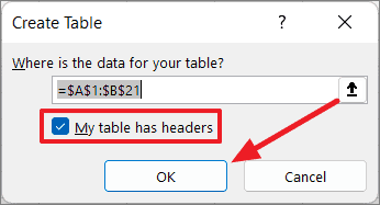
In the Create Table dialog box, confirm the range and click ‘OK’. If your table has headers, leave the ‘My table has headers’ option checked.
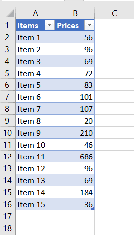
This will convert your data set into an Excel Table.
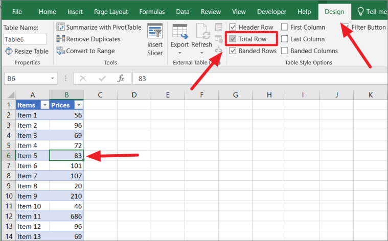
Once, the table is ready, select any cell within the table. Then, navigate to the ‘Design’ tab which only appears when you select a cell in the table and check the box that says ‘Total Row’ under the ‘Table Style Options’ group.
Once you have checked the ‘Total Row’ option, a new row would immediately appear at the end of your table with values at the end of each column (as shown below).
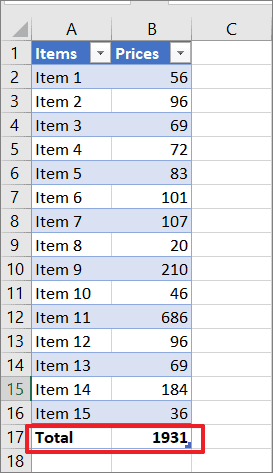
And when you click on a cell in that new row, you would see a drop-down next to that cell from which you can apply a function to get total. Select the cell at the last row (new row) of the column you want to sum, click the drop-down next to it, and make sure the ‘SUM’ function is selected from the list.
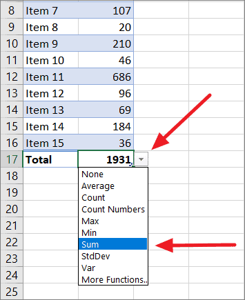
You can also change the function to Average, Count, Min, Max, and others to see their respective values in the new row.
Sum a Column Based on a Criteria
All the previous methods showed you how to calculate the total of the entire column. But what if you want to sum only specific cells that meet criteria rather than all of the cells. Then, you have to use the SUMIF function instead of the SUM function.
The SUMIF function looks for a specific condition in a range of cells (column) and then sums up the values that meet the given condition (or values corresponding to the cells that meet the condition). You can sum values based on number condition, text condition, date condition, wildcards as well as based on empty and non-empty cells.
Syntax of SUMIF Function:
=SUMIF(range, criteria, [sum_range])Arguments/Parameters:
range– The range of cells where we look for the cells that meet the criteria.criteria– The criteria that determine which cells need to be summed up. The criterion can be a number, text string, date, cell reference, expression, logical operator, wildcard character as well as other functions.sum_range(optional) – It is the data range with values to sum if the corresponding range entry matches the condition. If this argument is not specified, then the ‘range’ is summed instead.
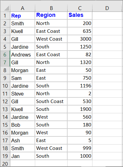
Suppose you have the below data set that contains sales data of each Rep from different regions and you only want to sum the sales amount from the ‘South’ region.
You can easily do that with the following formula:
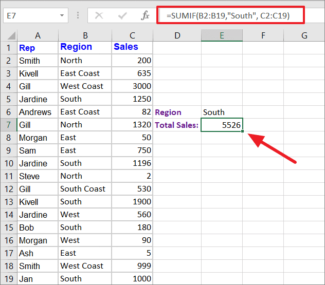
=SUMIF(B2:B19,"South",C2:C19)Select the cell where you want to display the result and type this formula. The above SUMIF formula looks for the value ‘South’ in column B2:B19 and adds up the corresponding Sales amount in column C2:C19. Then displays the result in cell E7.
You can also refer to the cell that contains text condition instead of directly using the text in the criteria argument:
=SUMIF(B2:B19,E6,C2:C19)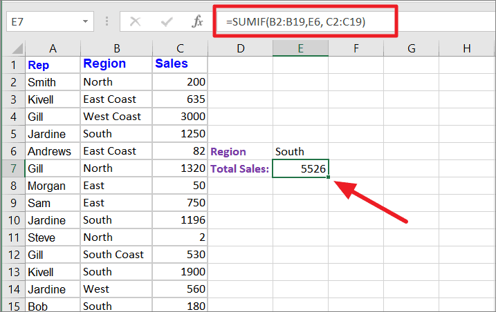
That’s it.


