
Conditional formatting in Excel allows you to automatically apply formatting—such as colors, icons, or data bars—to cells that meet certain conditions. This feature is invaluable for highlighting significant data points, emphasizing trends, or distinguishing anomalies within your spreadsheets.
By applying logical rules, Excel changes the appearance of cells based on their values relative to criteria you set. If a condition is met, the formatting is applied; if not, the cells remain unchanged. This dynamic formatting helps make data analysis more intuitive and efficient.
We’ll explore how to leverage conditional formatting to highlight cells or ranges based on specific conditions, enabling you to better interpret your data.
Highlighting cells with conditional formatting rules
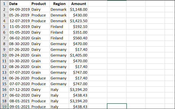
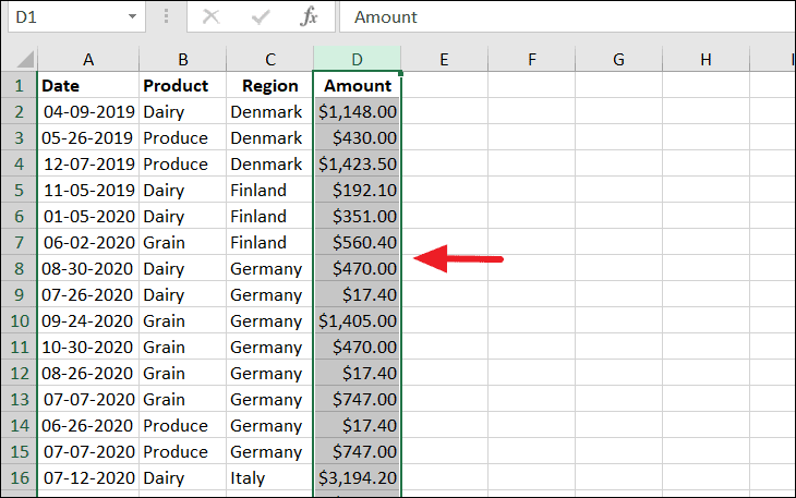
As an example, consider a worksheet containing sales records for various products. To easily identify sales amounts that are less than 500, you can use conditional formatting to highlight those values.
Home tab on the Excel ribbon. Click on Conditional Formatting in the toolbar to open the dropdown menu. Hover over Highlight Cells Rules, and then select Less Than... from the submenu. Excel provides several preset highlight rules you can choose from.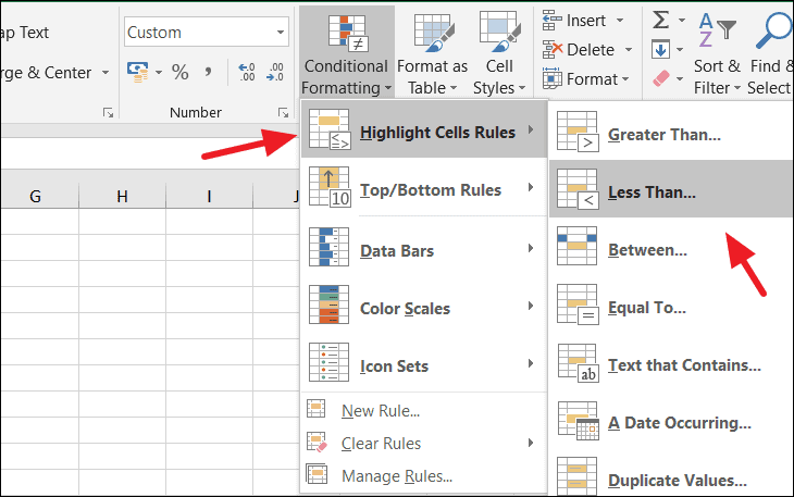
500 in the field that asks for the value. Choose the formatting style you prefer from the dropdown menu next to it. You can select from predefined formatting options or create a custom format.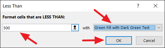
OK to apply the conditional formatting. All cells in column D with values less than 500 will now be highlighted according to the formatting you selected.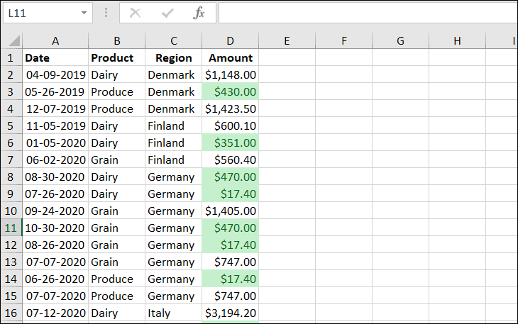
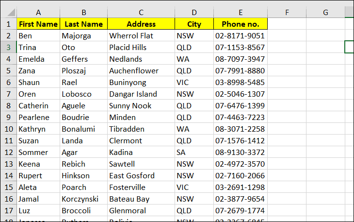
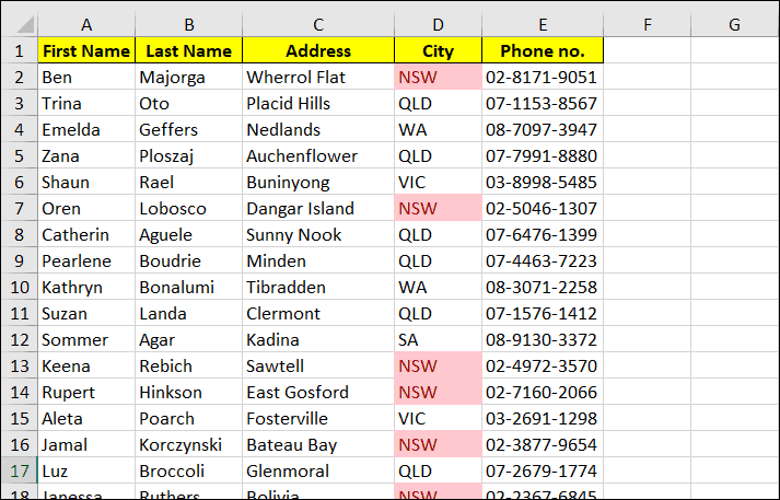
You can also use conditional formatting to highlight cells containing specific text. For example, suppose you want to identify all employees located in New South Wales (NSW).
Home tab, click Conditional Formatting, hover over Highlight Cells Rules, and choose Text that Contains...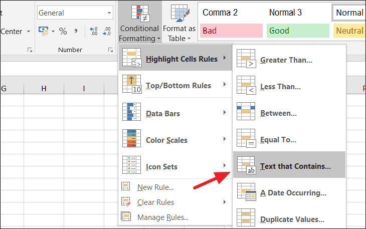
NSW in the text field. Select the desired formatting style from the dropdown menu, and click OK.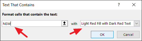
Now, all cells containing the text ‘NSW’ will be highlighted, making it easy to spot employees from that region.
Using top/bottom rules for conditional formatting
Excel’s top/bottom rules are invaluable for quickly identifying high or low values in your data set. These predefined rules enable you to highlight the top or bottom n items, top or bottom percentages, or values above or below the average.
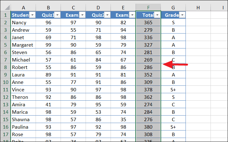
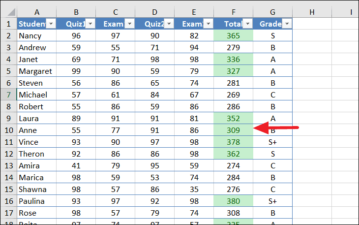
For instance, suppose you have a spreadsheet recording students’ exam scores, and you want to highlight the top 10 performers based on their total marks. Here’s how you can do it:
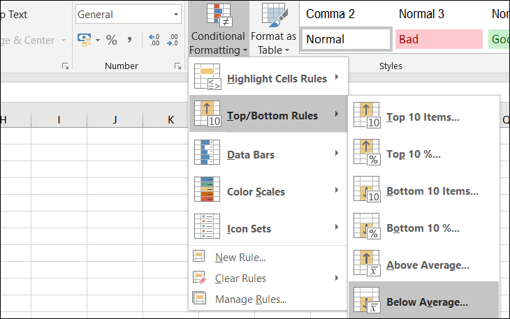
Home tab, click Conditional Formatting, hover over Top/Bottom Rules, and select Top 10 Items...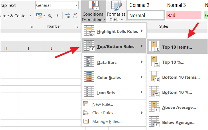
10, but you can adjust it using the arrows or by typing a number. Choose a formatting style from the list or create a custom format, then click OK.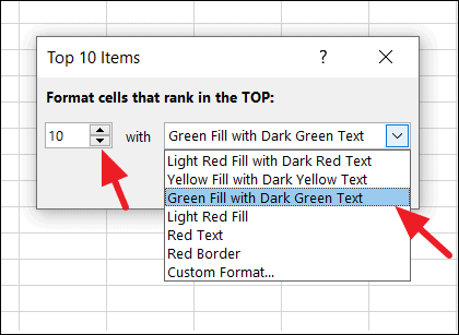
The top 10 values in the ‘Total’ column will now be highlighted, allowing you to quickly identify the highest-scoring students.
Similarly, you can highlight values that are above or below the average. For example, to find students who scored below average in ‘Exam 1’:
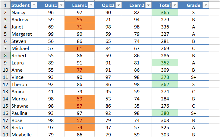
Custom Format... to create your own. For instance, you might choose an orange fill to highlight below-average scores. After selecting the format, click OK.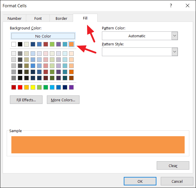
All cells with values below the average will now be highlighted with the chosen formatting.
Applying data bars
Data bars are a visual tool in Excel that represent the value of a cell relative to other cells with horizontal bars. The length of the bar corresponds to the cell’s value—a longer bar indicates a higher value, and a shorter bar indicates a lower value compared to the rest of the selected range.
Home tab, click Conditional Formatting, hover over Data Bars, and choose a style from the gradient or solid fill options.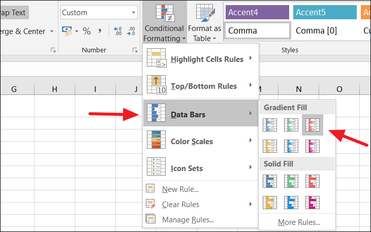
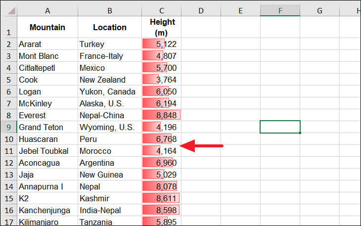
The data bars will appear within the selected cells, instantly comparing values across the range. Unlike other conditional formatting options, data bars display in all cells rather than only those that meet certain conditions.
Applying color scales
Color scales provide another method to visualize data by applying a color gradient to cells based on their values. Like data bars, color scales compare each cell’s value to others in the range, but instead of bars, they use a spectrum of colors to represent the data.
Color scales typically use two or three colors to represent the highest values, lowest values, and the in-between values. Cells with the highest values might be green, the lowest red, and mid-range values a shade of yellow, creating a visual gradient across your data.
Home tab, click Conditional Formatting, hover over Color Scales, and choose a color scale from the options provided.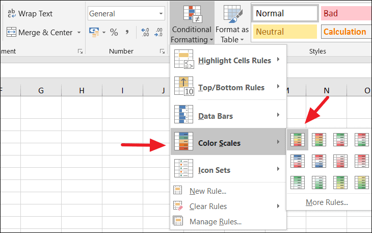
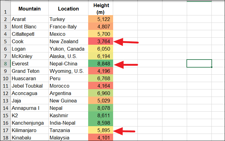
For example, choosing the red-yellow-green color scale will color the highest values green, the lowest values red, and the medium values yellow.
Applying icon sets
Icon sets offer yet another visual representation for your data by adding symbols to cells based on their values. These icons can be arrows, shapes, ratings, and more, providing immediate visual cues about the data.
Home tab, click Conditional Formatting, hover over Icon Sets, and select an icon style that suits your data. For this example, we’ll choose the first option under the ‘Directional’ category.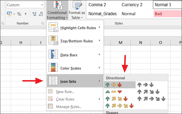
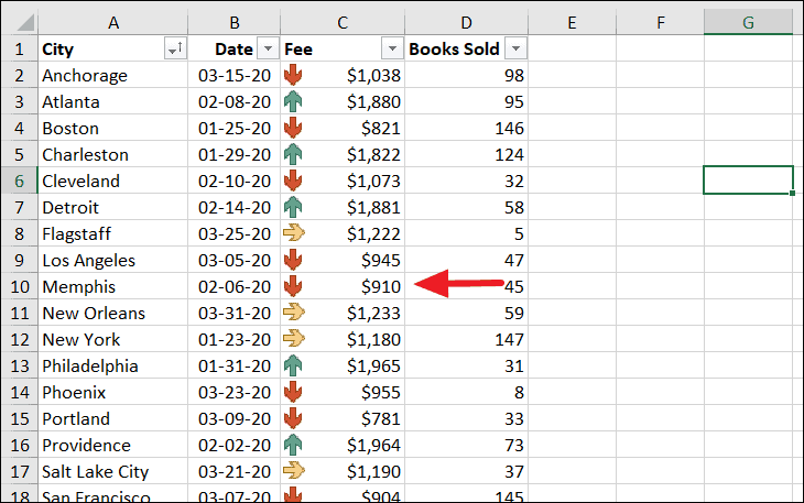
The icons will appear in the cells, representing the relative value of each cell. For example, green upward arrows may indicate higher values, yellow sideways arrows represent middle values, and red downward arrows signify lower values.
Removing conditional formatting
To remove conditional formatting from your worksheet, you can clear the rules applied:
Home tab, click Conditional Formatting, and select Clear Rules from the dropdown menu.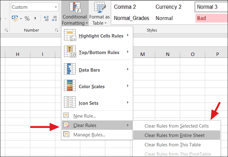
Clear Rules from Entire Sheet will remove all conditional formatting applied to the worksheet.By understanding how to apply and remove conditional formatting, you can enhance your data analysis in Excel, making important information stand out effectively.
Leveraging Excel’s conditional formatting allows you to dynamically highlight data, making it easier to analyze and interpret complex datasets. By mastering these tools, you can enhance your spreadsheets to be more informative and visually engaging.


