
The INDEX function is one of the most used functions in Excel that is categorized as a Lookup/Reference Function. The INDEX function is used to extract a value or reference of a cell in an array or range based on the row number and column number you specified. It can also be used to extract entire rows and columns in a table.
For instance, we have a table of 700 rows and 100 columns and we want to return the value at the 522nd row and 50th column. To do this you don’t need to scroll down hundreds of rows to get to the value, instead, you can use the INDEX function to return the value at the intersection of specified row and column number.
The INDEX function is often used with the MATCH function as a powerful alternative to the VLOOKUP. In the article, we will explain what the INDEX function is, how to use the INDEX function separately, and how to use INDEX and MATCH together with detailed examples in Excel.
Formats of INDEX Function
There are two formats of the INDEX function in excel: Array and Reference.
The Array form of the INDEX Function:
The array Index function is used to return the actual value(s) at the intersection of specified row and column in a single range.
Syntax:
=INDEX(array, row_num, [column_num])The arguments of the above function:
- array – This specifies an array or range of cells from which you want to return a value from.
- row_num – This specifies the row number from which you want to extract the value.
- column_num – This specifies the column number from which you want to extract the value. If it is omitted or zero, the function takes 1 as default.
If the row number is not specified, the column number is required and if the column number is omitted, the row number is required.
The Reference format of the INDEX Function
The Reference format of the INDEX function is used to return the reference of the cell at the intersection of row number and column number.
Syntax:
=INDEX(reference, row_num, [column_num], [area_num])The function uses the below arguments:
- reference – This argument specifies the reference to one or more cell ranges (areas). If multiple ranges or arrays are used in a function, they need to be separated by commas and closed by brackets i.e. (A3:B11, B15:D5, E10:K50).
- row_num – It denotes the row number in the specified reference or array.
- [col_num] – It denotes the column number in the specified reference or array. If it is omitted or zero, the function takes 1 as default.
- [area_num] – If the reference argument is made up of multiple ranges or arrays, this specifies which range or area to use. The areas are numbered left to right in the reference argument. The first area entered is considered 1, the second 2, and so on. If this argument is omitted, it defaults to the value 1.
How to Use INDEX function in Excel
To better understand how the INDEX function works in Excel, let’s consider a few examples.
INDEX Function with One-Dimensional Array (Array Format)
The INDEX function can be used on a One-dimensional array (one-way lookup) to return value from a single row or column. For this function, only the array argument and row number or column number are required.
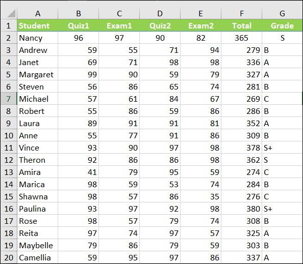
Let’s assume you have the below dataset:
Now, select the cell where you want to return the result of the function. Then, type the following formula to get the 10th-row mark of Exam 1 and press Enter:
=INDEX(C2:C20,9)In the above formula, C2:C20 specifies the range or column and 9 refers to the row number to fetch the value from the given range. Since we are looking up the value in a single column, the col_num argument is omitted.
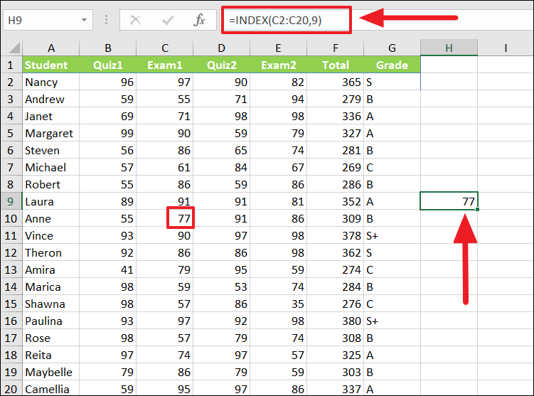
As you can see above, we excluded column heading when we specified range in the formula, so we can start counting the row from C2 i.e. 1st row in the given range, hence the value at row 9 is 77.
INDEX Function with Two-Dimensional Array (Array Format)
The Two-dimensional array means an array with more than one row and one column. To use the array function in a two-way lookup, you will need a range, row number, and/or column number. If a row number or column number is ignored, it defaults to 1.
Suppose we have the below dataset where we want to look up and return Laura’s score in Quiz 2.
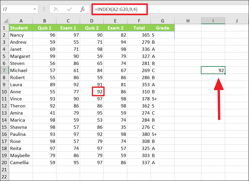
To do that, select the cell where you want to return the result and execute the following formula:
=INDEX(A2:G20,9,4)Where A2:G20 (column heading excluded) is the table or range, 9 is the row number and 4 is the column number in the formula. The above formula returns the value (92) at the intersection of row 9 and column 4 in table A2:G20.
INDEX Function with Only Row or Column Number (Array Format)
If an array argument contains multiple rows and columns, we need to specify both the row and column numbers to fetch a specific value. However, if the row or column number is left empty or entered as zero in the INDEX formula, the formula returns an array of values.
Example 1:
Try the below formula where the column number is zero or blank:
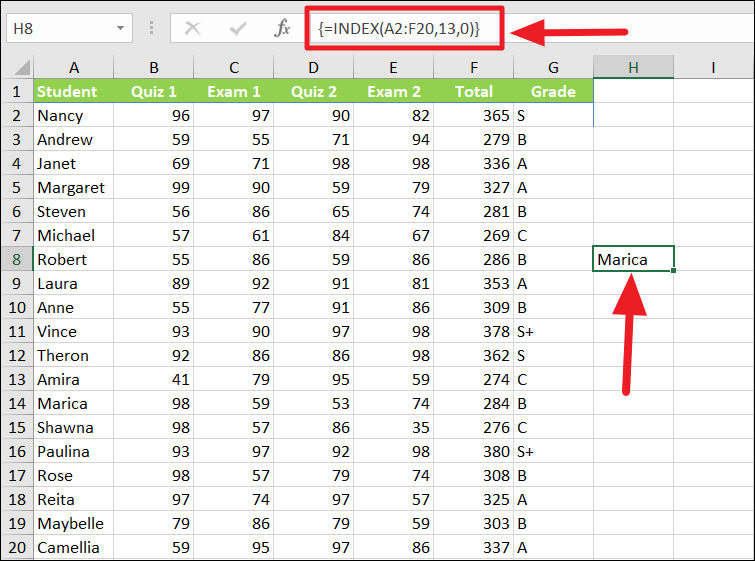
=INDEX(A2:F20,13,0)or
=INDEX(A2:F20,13,)When a formula returns multiple values, it is considered an array formula. So it must be executed by pressing Ctrl+Shift+Enter. So, type the above formula and press Ctrl+Shift+Enter to run it as an array formula.
If the INDEX formula is entered as an array formula in a single cell, it only returns the first value in the specified row or column as shown below. If a formula is executed as an array formula, the curly brackets will be automatically inserted.
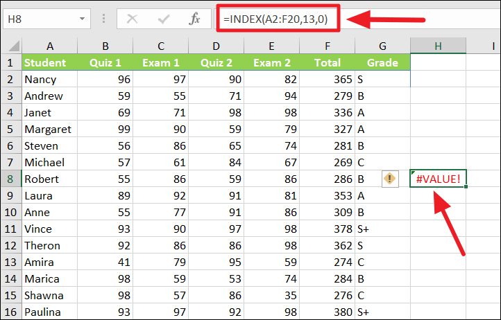
In case, either row number or column numbers or both are entered as zeros or blank, and you execute the formula as a normal formula by simply pressing Enter, the output would ‘#VALUE!’ error.
Example 2:
Before entering the INDEX formula as an array formula, first, you need to select the exact output range. The output range should have the same number of empty cells as the array of the source dataset. Here’s how you do this:
To return an array of values as an output from the INDEX formula, first, select the blank output range A23:G23. Then, type the formula =INDEX(A2:F20,13,0) in the first cell selected (A23) and press the Ctrl+Shift+Enter simultaneously to execute it as an array formula.
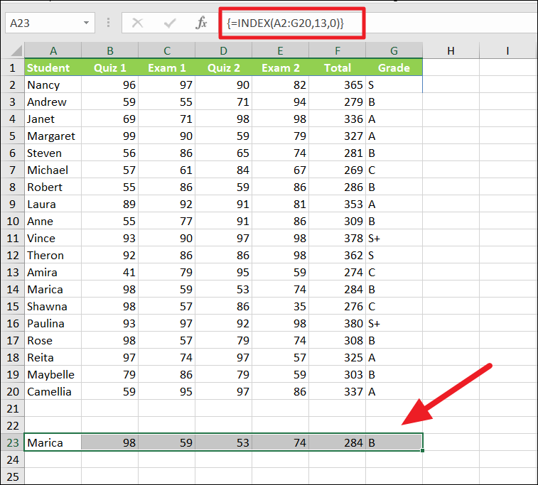
As you can see above, the entire row is returned as output in the selected range.
Example 3:
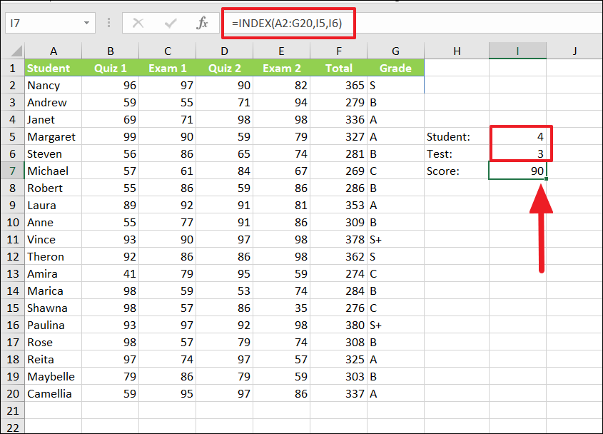
You also can use the cells to input your Row number and Column number to get dynamic results from the INDEX formula, without having to change your formula every time to get a different output.
To accomplish this, use the below formula:
=INDEX(A2:G20,I5,I6)Where A2:G20 is the range, I5 reference tells the formula to use the value in that cell as row number and I6 refers to the value in that cell as the column number to return the result (86).
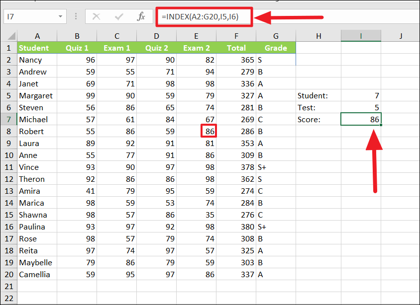
Now you can easily adjust the row or column number in cells I5 and I6 to fetch a different result without making any adjustment to the original formula.
INDEX Function with Multiple Arrays (Reference Form)
INDEX Reference Form can be used to extract value if you have multiple arrays or tables in the formula. You can also use a single cell reference not just an array in the formula. Reference Form INDEX Function also needs an additional argument – Area number which tells the function from which array to pull data.
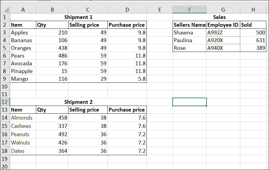
Suppose, you have three different datasets that contain sales and shipment details of products as shown below.
To extract value from multiple two-dimensional arrays with Index, type below formula where you want the result and press Enter:
=INDEX((A3:D9,A14:D18,F3:H5),3,4,2)Here, A3:D9, A14:D18, F3:H5 are the 3 areas of the reference argument and they are referred to as Area 1, 2, and 3 respectively. The row number and column number are 3 and 4 respectively, from where we need to fetch the value. And the final argument 2 specifies which range or area to use.
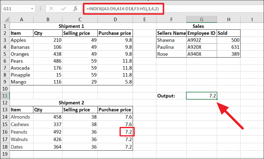
As a result, the INDEX formula will output the value from the 3rd row of the fourth column from the 2nd array in the sheet i.e. ‘7.2’.
Index Function with Other functions
The Index function can be used with various other functions to make various calculations in Excel.
Example 1:
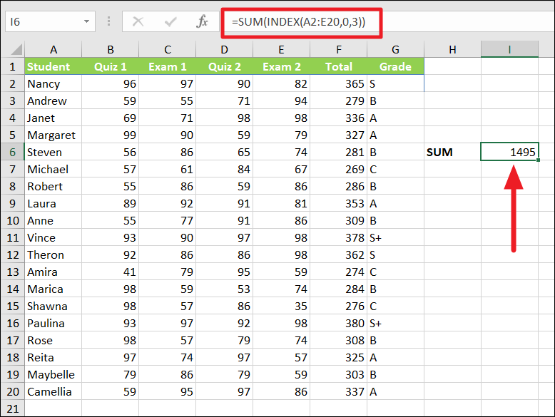
For instance, we want to sum the values of the 3rd column of table A2:C20 with the help of the INDEX function. You can do that with below formula:
=SUM(INDEX(A2:E20,0,3))Here, the INDEX function is enclosed within the SUM function to sum the values of the 3rd column.
Example 2:
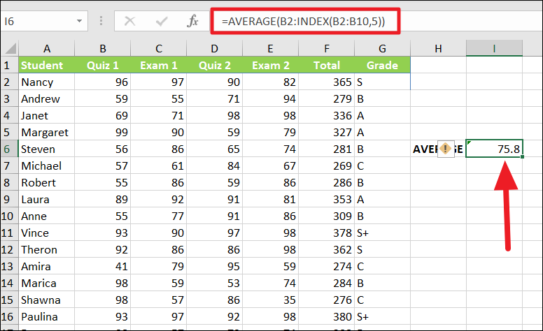
Let’s try the INDEX function with an average formula to return the average of a range. By default, the Index function returns the value of a cell. However, when the INDEX function comes after cell reference and colon (:), it will return a cell reference instead.
For instance, the below formula returns the average of the cell range B2:B6:
=AVERAGE(B2:INDEX(B2:B10,5))The INDEX(B2:B10,5) returns a reference to cell B6 because a cell reference and colon (:) was preceding the function. As a result, now we have the formula AVERAGE(B2:B6) and the output is 75.8.
If you change the row numbers in the INDEX function, it will produce dynamic results.
Using INDEX and MATCH Finctions Together
INDEX functions are rarely used alone. They are often paired with MATCH to make powerful calculations. When the INDEX function is combined with the MATCH function, it can perform advanced left lookups. Many people still prefer using VLOOKUP to lookup a value, because it’s more popular and simpler but INDEX MATCH is more flexible and faster than VLOOKUP.
Unlike the VLOOKUP function, it can work with data that are arranged both vertically and horizontally and it can lookup values from left to right as well as the right to left. INDEX MATCH has no array restriction and lookup value size limit. Moreover, INDEX and MATCH use dynamic data ranges when looking up values.
Excel MATCH Function
Before we combine the INDEX and MATCH functions, first, let us see how the MATCH function works with an example.
The MATCH function is a built-in function in Excel that searches for a specific value in a range of cells and returns the relative position of that value in the given range.
Syntax of MATCH Function:
=MATCH(lookup_value,lookup_array,[match_type})Where:
lookup_value – The value you want to look up in a specified range of cells or an array. It can be a numeric value, text value, logical value, or a cell reference that has a value.
lookup_array – The arrays of cells in which you are searching for a value. It must be a single column or a single row.
match_type – It is an optional parameter that can be set to 0,1, or -1 and the default is 1.
- 0 looks for an exact match, when it’s not found, returns an error.
- -1 looks for the smallest value that is greater than or equal to lookup_value when the lookup array is in ascending order.
- 1 looks for the largest value that is less than or equal to the look_up value when the lookup array is in descending order.
Example:
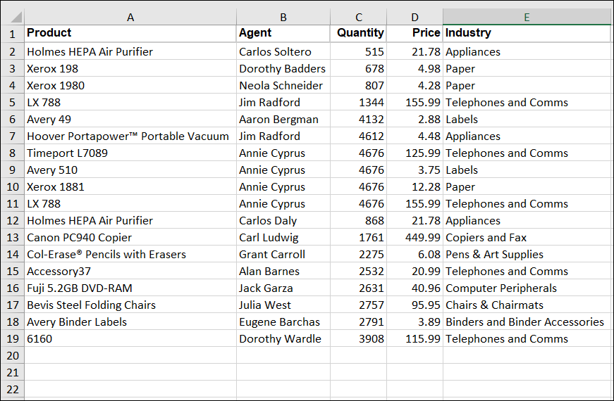
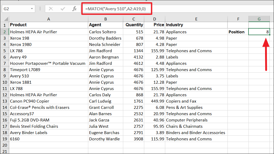
In the below dataset we want to find the exact position of the product name (Avery 510), let us see how we can do that with the MATCH function.
To find the position of the value in a row or column, try the below formula:
=MATCH("Avery 510",A2:A19,0)In the above formula, Avery 510 is the lookup value we want to find the position for, A2:A19 is where to look for the value, and 0 tells the function to look for the exact value. As a result, the formula returns the position of the value as ‘8’ in the given range.
The MATCH function is case-insensitive, it doesn’t matter if the lookup value is in lower case or upper case, it will find the exact value. If the lookup value is a string, it must be enclosed in double-quotes.
You also can use the cells to input your lookup value to get dynamic results, without having to change your formula every time you want a different output. For that, use a cell reference that contains the lookup value in the first argument.
The following formula finds the position of the value in the cell G2:
=MATCH(G2,A2:A19,0)
Combine INDEX and MATCH function
VLOOKUP can only look up a value vertically i.e columns while INDEX MATCH combo can do both vertical and horizontal lookups.
The INDEX function is used to fetch a value at a specific location in a table or a range while the MATCH function returns the relative position of a value in a column or a row. When combined, the MATCH can find the row or column number (position) of a specific value, and the INDEX function can retrieve the value based on that row or column number.
Example:
Suppose, we have the below dataset as shown below:
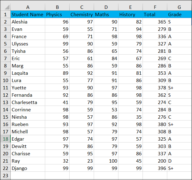
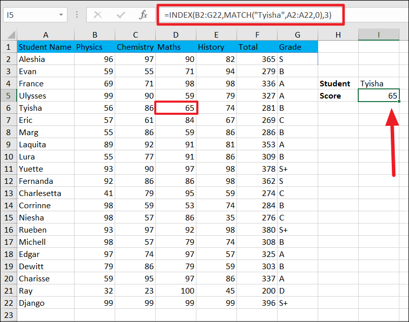
In the above table, let’s say you want to retrieve the ‘Maths’ score for the student named ‘Tyisha’, try the below formula:
=INDEX(B2:G22,MATCH("Tyisha",A2:A22,0),4)In the above formula, the nested MATCH function finds the row number (position) of the value ‘Tyisha’ (5). Then that row number and a column number (4), which we specified as the last argument is supplied to the INDEX function. As a result, the formula retrieves the values at the intersection of row (5) and column (4) numbers within the table B2:G22 and returns the score ’65’.
You can also use cell reference as an argument for the lookup value in the formula:
=INDEX(B2:G22,MATCH(I4,A2:A22,0),4)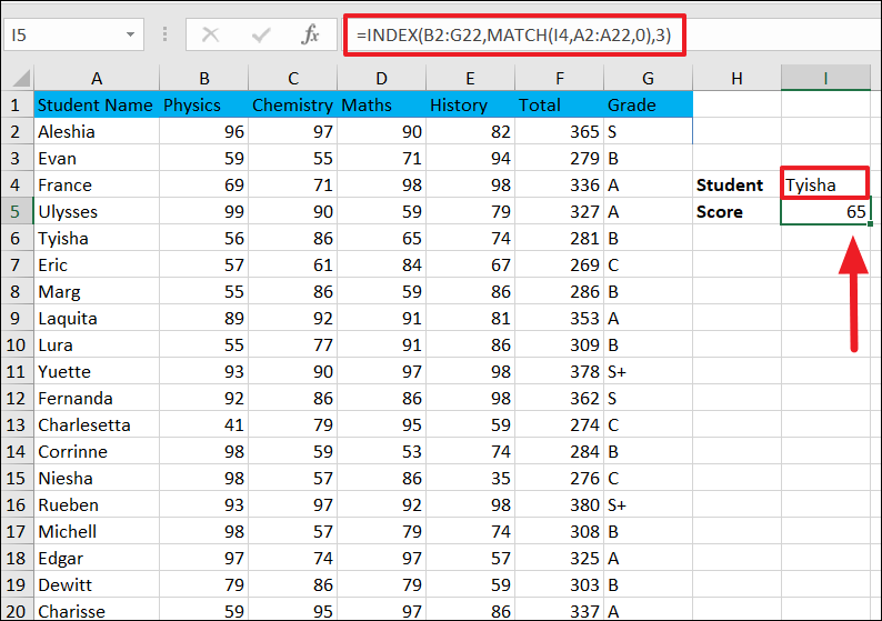
Two-way lookup with INDEX and MATCH
In the above example, we know the column number (manually entered) and we only used the MATCH function to find the row number to retrieve data. But let’s assume, we don’t have the column number either and we only know the row (student name) and column heading (subject) to go by. In that case, you can use the INDEX and MATCh functions to find a value with a two-way lookup (two-dimensional array).
For this, we need to nest two MATCH functions within the INDEX function: One for row number and one for column number.
Example 1:
Now, we want to find out how many marks ‘Lura’ scored in the ‘History’ subject. Here’s how we can do that:
To apply a two-way lookup with INDEX and MATCH, you can use the below formula:
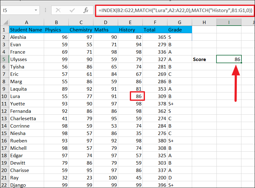
=INDEX(B2:G22,MATCH("Lura",A2:A22,0),MATCH("History",B1:G1,0))As we know, the MATCH function can look for a value both horizontally and vertically. In this formula:
- MATCH(“Lura”,A2:A22,0) looks for the value ‘Lura’ vertically in the range A2:A22 and returns its position, which is the row number (9).
- MATCH(“History”,B1:G1,0) looks for the value ‘History’ horizontally in the range B1:G1 and returns its position, which is the column number (4).
Then both row and column number is supplied to the INDEX function to retrieve the score (86) at the intersection in table B2:G22.
Dynamic Two-way Lookup with INDEX and MATCH
If you have large data, you may want to make the lookup values dynamic in the Match function, so you don’t have to manually enter lookup values in the function. You can simply update the lookup values in specific cells so that the MATCH functions can automatically identify values in the specified cells and return exact positions (row and column number).
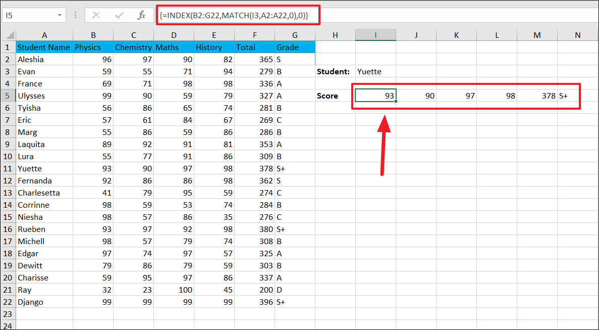
Here is the formula for a fully dynamic, two-way lookup with INDEX and MATCH:
=INDEX(B2:G22,MATCH(I3,A2:A22,0),MATCH(I4,B1:G1,0))In the above formula, MATCH(I3,A2:A22,0) returns a dynamic row number by identifying the value in cell I3 and searching for it in the range A2:A22. The MATCH(I4,B1:G1,0) returns a dynamic column number by identifying the value in the cell I4 and looking for it in the range B1:G1. Then both values are supplied to the INDEX function to retrieve Yuette’s score in Chemistry: 90.
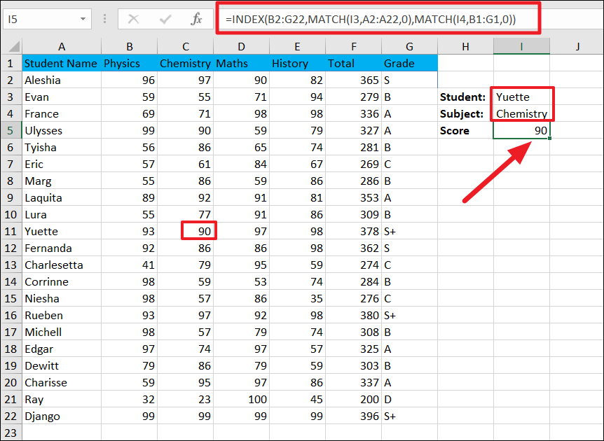
You can change the student name and/or subject in the cells ‘I3’ and ‘I4’ to get different dynamic results.
Example 2:
If you want to get values from an entire row or column instead of a single cell value. For example, we can use the INDEX MATCH formula to get all the scores of ‘Yuette’ including the scores in all the subjects, their total, and grade.
To do that, try the below formula:
=INDEX(B2:G22,MATCH(I3,A2:A22,0),0)First, select the output range with as many cells as in the source range, type the formula, and press Ctrl+Shift+Enter. Here, we used 0 as the column number. As a result, we got an array of outputs as shown below.
If you want to see the array output the formula returns, simply select the formula in the edit mode and press F9.
Suppose we don’t have total marks in the above table, we can get total marks of ‘Yeutte’ in all four subjects by nesting the above formula within a SUM function.
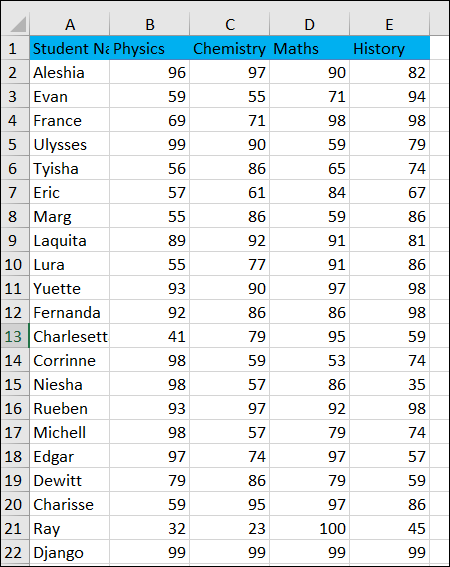
Here are the scores of all the students in four subjects.
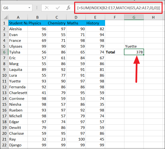
Now, type the below formula and run it as an array formula ( Ctrl+Shift+Enter ):
=SUM(INDEX(B2:E17,MATCH(G5,A2:A17,0),0))Here, the INDEX and MATCH functions return scores in all four subjects for Yeutte and the SUM function sums them up and outputs the total as 378.
Similarly, you can use the MAX function with INDEX to calculate the highest score and the MIN function to find out the lowest score.
Create Drop Down Lists to Input Values for INDEX and MATCH formula
In the above examples, we had to hardcode the lookup value in the MATCH function or enter the lookup value in the specified cells to make the formula dynamic. However, if you have a huge dataset, this could be a time-consuming and error-prone process (if you misspell or specify the wrong value.
You can easily avoid this by creating a drop-down list of lookup values (Student names and subjects), and selecting a value from the drop-down list. After choosing a value, the formula would automatically update the output. Here’s how you do this:
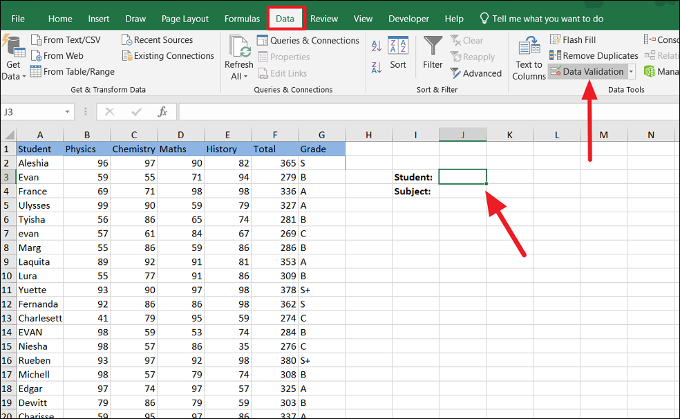
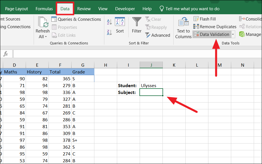
First, select the cell where you want to create the drop-down. Here, we want the student names drop-down list in ‘I3’. Then, go to the ‘Data’ tab and click the ‘Data Validation’ button in the Data Tools group.
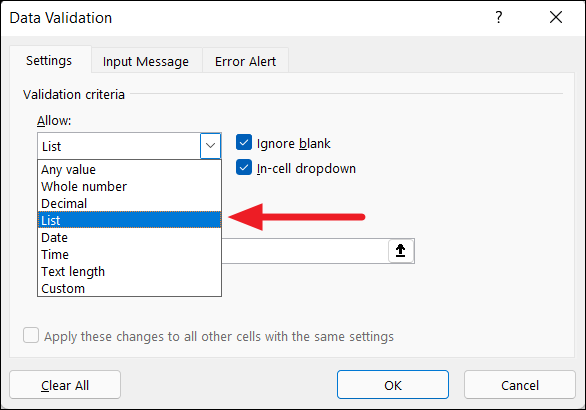
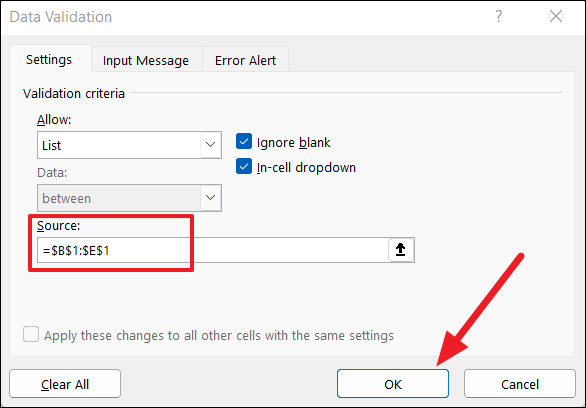
In the Data Validation Dialogue box, go to the Settings tab, and choose ‘List’ from the ‘Allow:’ drop-down.
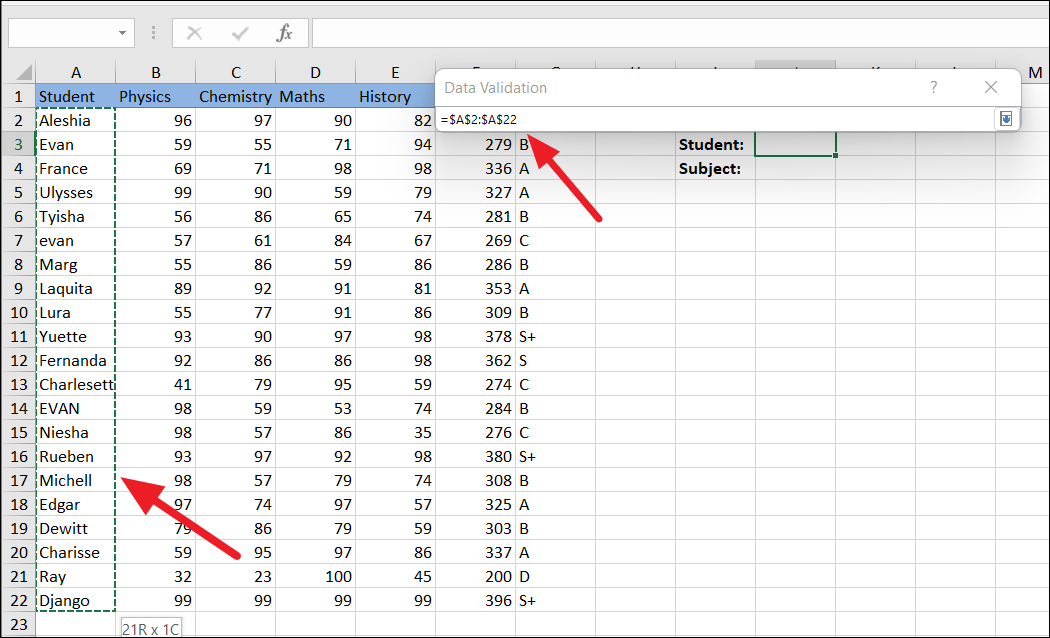
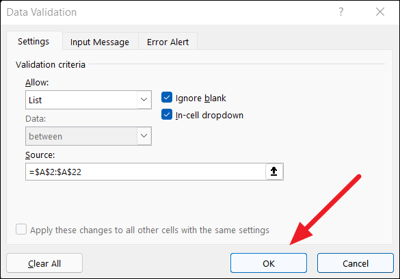
Next, click on the ‘Source’ field and select the range with the Student names: ‘$A$2:$A$22’.
Then, make sure both ‘Ignore blank’ and ‘In-cell dropdown’ options are selected and click ‘OK’.
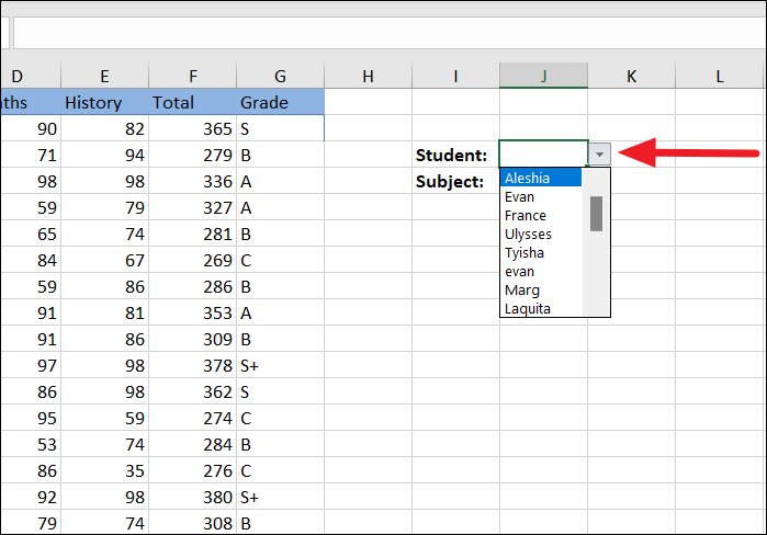
This will create a drop-down in the selected cell as shown below. Remember, the drop-down menu will only be visible when you select that cell. You can select the cell and click the drop-down button to view the list of names.
Now, repeat the same steps to create a drop-down list for subjects. To do that, select a cell where you want the ‘Subjects’ drop-down list. Next, go to the ‘Data’ tab and click the ‘Data Validation’ button in the Data Tools group.
From the Data Validation Dialogue box, choose the ‘List’ option from the ‘Allow:’ drop-down in the Settings tab. After that click on the Source field and select the range with subjects ($B$1:$E$1). Then, click ‘OK’.
This will create a drop-down for subjects in the selected cell.
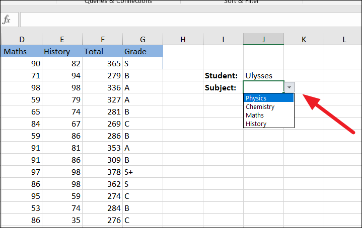
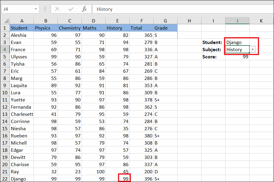
Now, select the student name and subject from those drop-down lists.
After that, you need to enter a formula that gets input values from the drop-down lists. For that, try the below formula, which is nearly the same as the one we used in the Dynamic two-way lookup example:
=INDEX(B2:E22,MATCH(J3,A2:A22,0),MATCH(J4,B1:E1,0))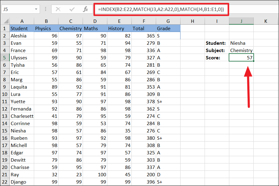
Now, you don’t have to hardcode lookup values into the formula or in the input cells, you can simply select the name and subject from the drop-down lists and it will automatically update the results.
Three-Way Lookup with INDEX/MATCH Formula (Reference form)
You can also use the INDEX and MATCH formula to retrieve a value with a three-way lookup. In the above example, we used a two-way dynamic lookup (two lookup values) to get student scores from a table.
In the above examples, we’ve used one table with scores for students in different subjects. This is an example of a two-way lookup as we use two variables to fetch the score (student’s name and the subject).
Example:
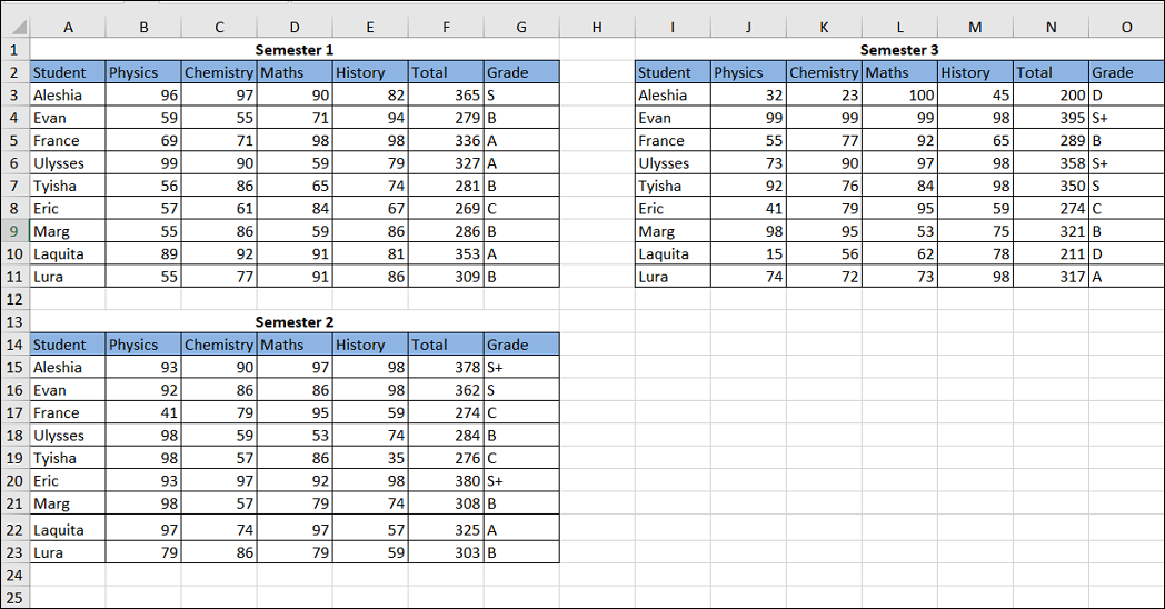
But, what if you want you to want to fetch a student score in a certain subject from a specific semester? For instance, let’s assume you have three tables (each for a different semester) with lists of students and their scores on different subjects.
Now, you can use the combination of INDEX and MATCH to fetch a student’s score for a particular subject from the specific semester using the three-way lookup. For a three-way lookup, you need three inputs, row number (student name), column number (subject), and area number (Semester).
First, we need to create three drop-down menus, one for student names, another for subjects, and another for semesters. Create the students and subjects drop-downs, the same way you did for the previous example. For the semester drop-down, you need to enter the semester names in an empty range and use that to make a drop-down.
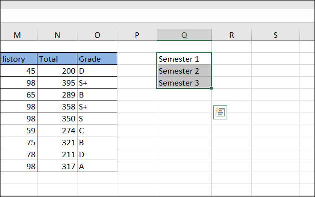
To do that, enter the semester names in a range of cells, then select the cell where you want the drop-down and go to Data –> Data Tools –> Data Validation.
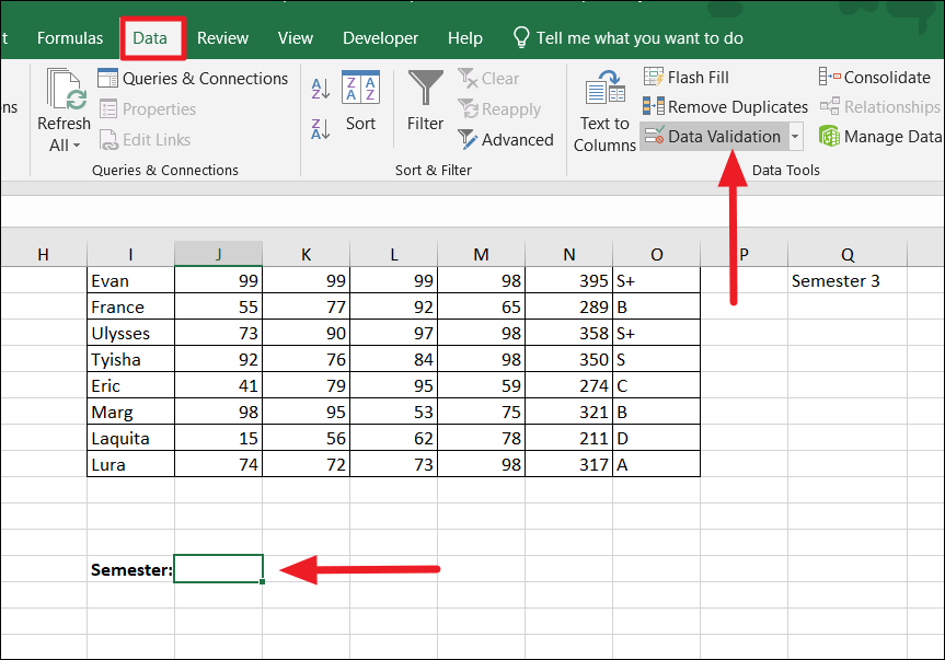
In the Data Validation dialog box, choose List for Validation criteria, select the range with semester names, and click ‘OK’
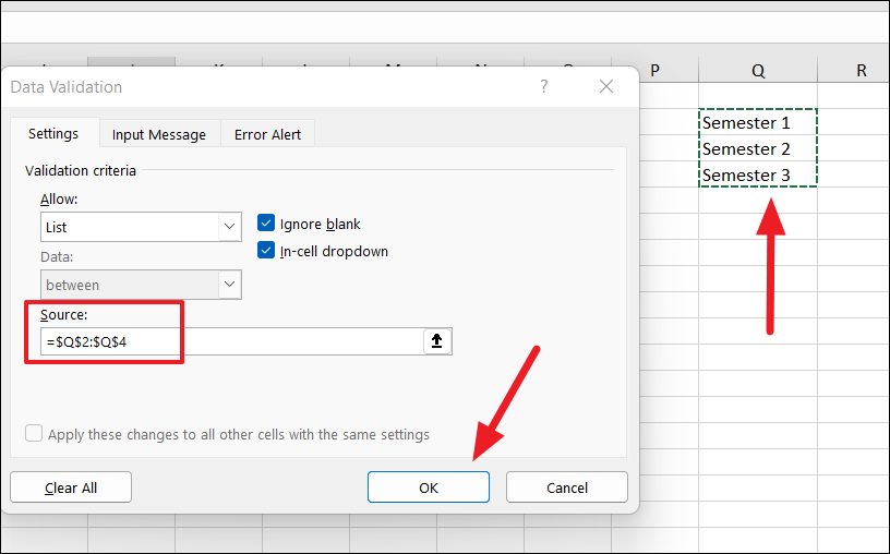
Now, the semester drop-down is created.
Similarly, create drop-downs for Student names and subjects. Then, select a cell where you want the output and enter the following formula:
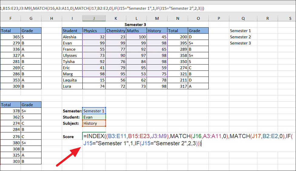
=INDEX((B3:E11,B15:E23,J3:M9),MATCH(J16,A3:A11,0),MATCH(J17,B2:E2,0),IF(J15="Semester 1",1,IF(J15="Semester 2",2,3)))Since it’s a big formula, let us break it down for you:
(B3:E11,B15:E23,J3:M9)are the reference for the arrays (table for each semester). When specifying multiple arrays, they must be enclosed in parentheses.MATCH(J16,A3:A11,0)is the MATCH formula used to find the row number of the student’s name from the drop-down list in cell J16.MATCH(J15,B2:E2,0)is the MATCH formula used to find the column number of the subject from the drop-down list in cell J17.IF(J15="Semester 1",1,IF(J15="Semester 2",2,3)))is the area number argument which informs the INDEX function which table to search for the value. If ‘Semester 1’ is selected in the drop-down list, it returns 1. If that’s false, it checks for ‘Semester 2’ and returns 2 and if that is also false, it returns 3.
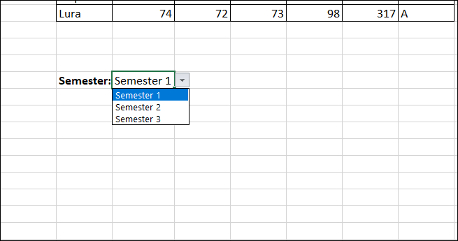
Then, choose the semester, student, and subject from the drop-down menus to fetch a particular student’s mark for a particular subject in the selected semester.
The result:
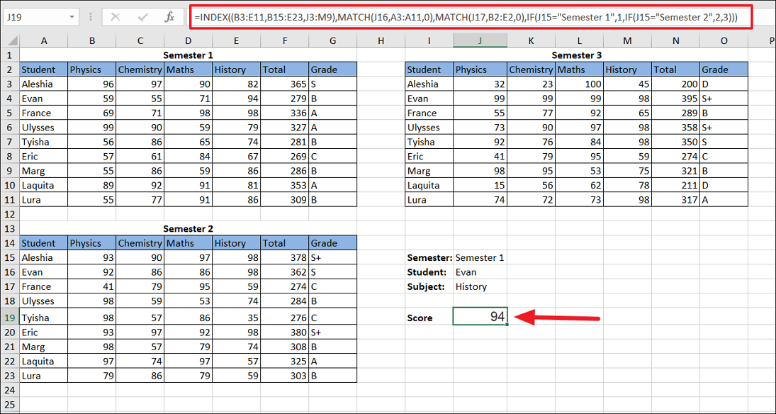
Now, whenever you choose a different option in the drop-down, the output will auto-adjust.
Left Lookup using INDEX and MATCH
Unlike the VLOOKUP function, the INDEX and MATCH function can look to the Left and extract value from the left side of the column that has the lookup value.
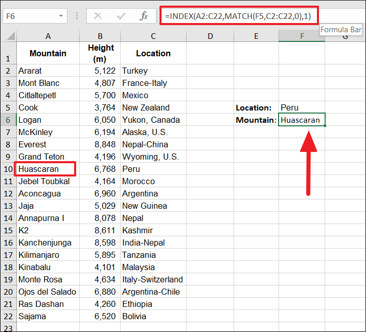
For example, in the below dataset, we have the list of mountains, their height, and where they are located. Now, we have the location as the lookup value and we want to find out which mountain is located there. Here’s how you can do that with the INDEX MATCH combo by looking from right to left.
Select the cell where you want the output, and enter the below formula:
=INDEX(A2:C22,MATCH(F5,C2:C22,0),1)In the above formula, the MATCH function searches for the lookup value (F5) in the range C2:C22, and when a match is found, it retrieves the corresponding in the 1 st column to the left.
Case-Sensitive Lookup with INDEX and MATCH
By default, the INDEX and MATCH combo is not case-sensitive. It doesn’t matter what case is the lookup value is, it returns the same output. For instance, if you search for ‘Dexter’, ‘dexter’, or ‘dEXteR’, all the lookup values will return the same position number.
However, if you have a list of student’s test scores and multiple students with the same name, you can use the EXACT function within the INDEX function to distinguish upper-and-lower-case characters.
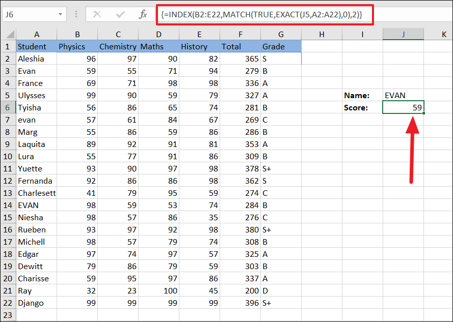
To perform a case-sensitive lookup using the INDEX and MATCH, use the below formula:
=INDEX(B2:E22,MATCH(TRUE,EXACT(J5,A2:A22),0),2)This is an array formula, so enter the above formula and press Ctrl+Shift+Enter otherwise you’ll get N/A! error.
The table below contains three Evans (Evan, even, EVAN). The Exact function checks each value in the range A2:A22 against the lookup value in cell J5 (EVAN) for an exact match. When an exact match is found, it returns TRUE and the MATCH function returns that position as the row number (13). And the column number is specified in the last argument as ‘2’. As a result, we get the score for EVAN in chemistry as 59.
Although we used cell reference for the lookup value, you can also hardcode the lookup value directly into the formula.
Multiple Criteria Lookup with INDEX and MATCH
With INDEX and MATCH functions, you can perform a lookup based on multiple criteria. In this method, to look up a value, the MATCH function must meet criteria in 2 or more columns at the same time.
For instance, if you have a large database and you want to look up the name ‘John’. But the problem is multiple records have the same first name ‘John’. This might cause problems as you might fetch up the wrong value. To fix this, you can use an INDEX and MATCH function that can look up a value that matches on more than one column (multiple criteria) and retrieve the corresponding value.
The syntax for INDEX MATCH with multiple criteria:
=INDEX(return_range, MATCH(1, (criteria1=range1) * (criteria2=range2) * (…), 0))where,
- return_range is the range from which the value will be fetched
- criteria1, criteria2, … are the criteria that should be met
- range1, range2, … are the ranges on which the required criteria should be tested.
Example:
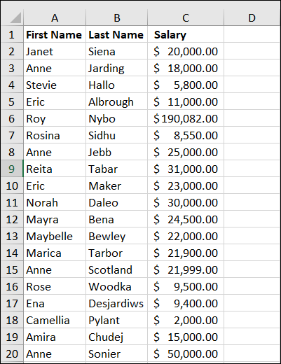
In the below dataset, we want to retrieve the salary for ‘Anne’ but we cannot look for ‘Anne’ because there are three differnt records with ‘Anne’ as the first name.
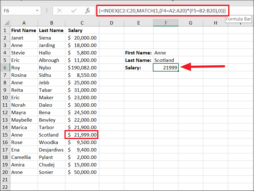
The below formula looks up and returns salary for the record that has the first name ‘Anne’ and the last name ‘Scotland’ (multiple criteria):
=INDEX(C2:C20,MATCH(1,(F4=A2:A20)*(F5=B2:B20),0))This is an array formula, so make sure to run it by pressing Ctrl+Shift+Enter.
Here, the MATCH function checks for the first name ‘Anne’ (F4) in column A2:A20 and the last name ‘Scotland’ (F5) in column B2:B20. If both columns match the specified lookup values, it returns the corresponding salary from column C2:C20.
Find the Closest Match with INDEX and MATCH
Finding exact value with INDEX and MATCH is easy but finding a closet match to a specific value in the range is a bit complicated and it involves two more functions ABS and MIN along with the INDEX and MATCH.
For instance, if you have a list of events and their dates in a table and you want to find an event that is closest to a specific data, you can use the following example.
To find the closest match to a specific value in a column, use the below formula syntax:
{=INDEX(data,MATCH(MIN(ABS(data-value)),ABS(data-value),0))}Where
datais the range of input values.valueis the input value to which the output will be closest.MINfunction is used to return the smallest value from the array of data values.ABSreturns the absolute value of a number.1( exact or next smallest ) or0( exact match) or-1( exact or next largest )
Example:
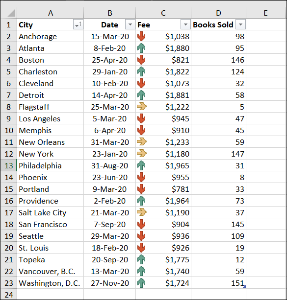
Let’s assume you have the below dataset and you want to look for the date which is closest to the given date and fetch the corresponding city name.
To find the closest date to March 25, 2020, in the range, try the below formula:
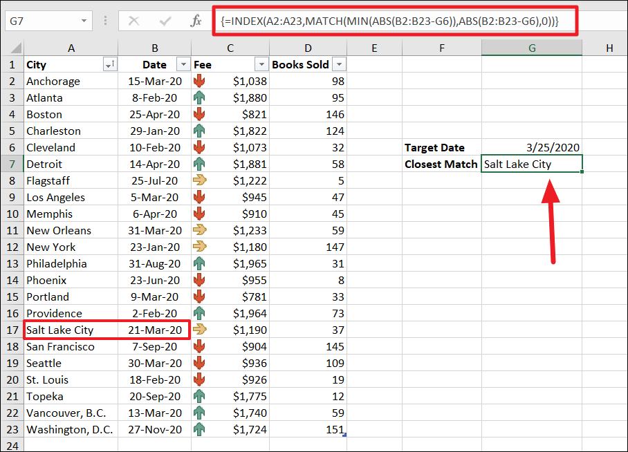
=INDEX(A2:A23,MATCH(MIN(ABS(B2:B23-G6)),ABS(B2:B23-G6),0))Then, press Ctrl+Shift+Enter to execute the formula as an array formula.
In the above formula, ABS(B2:B23-G6) finds the difference between the search array (B2:B23) and the given date by subtracting all date values from the specified date in cell G6. This creates a returned array with the subtracted values. Then, MIN(ABS(B2:B23-G6) finds the closed value from the subtracted values. Then, the MATCH function finds the position of the closed minimum value in the array constant and that position number is returned to the INDEX function as the row number.
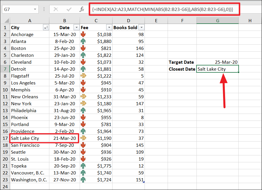
As a result, the INDEX function returns the corresponding city name for the closet date.
Wildcard Match with INDEX and MATCH
Wildcards can be used in the INDEX and MATCH function combo can be used to find a value with a partial match. It can work only when match_type is set to ‘0’ and the lookup value is a text string in the MATCH function. There are wildcards you can use in the MATCH function: an asterisk (*) and a question mark (?).
- Question mark (?) is used to match any single character or letter with the text string.
- Asterisk (*) is used to match any number of characters with the string.
For example, below is a dataset of products, their quantities, and prices.
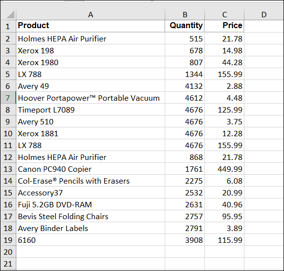
Suppose you want to get the price for a specific product but you only know the partial name of the product. You can still get the right data by using a wildcard character with the lookup value. You can use the asterisk (*) wildcard to match any number of characters while a question mark (?) is used to match any single character.
Asterisk (*)
You can try the below formula to achieve this:
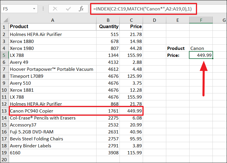
=INDEX(C2:C19,MATCH("Canon*",A2:A19,0),1)or
=INDEX(C2:C19,MATCH(F4&"*",A2:A19,0),1)Where the MATCH function searches for the value that starts with ‘Canon’ followed by any of the characters, in the Product column (A2:A19). This means that “Canon* in the lookup argument means any text string that starts with the word ‘Canon’ and can have any number of characters after it.
In the below table we have ‘Canon PC940 Copier’ in the range, so it returns the row number (12) to the INDEX function. Then, the INDEX function retrieves the value from the 12th row in the Price range (C2:C19).
Question mark (?)
You can use the question mark (?) wildcard to represent any single missing character in the string.
To find a value that matches the text string with any single character (in the wildcard place):
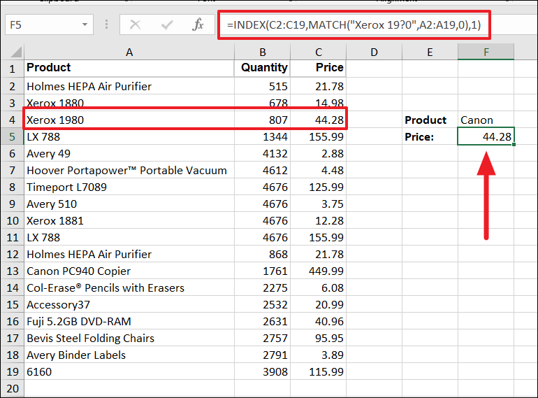
=INDEX(C2:C19,MATCH("Xerox 19?0",A2:A19,0),1)Here, the MATCH formula looks for the Xerox 19?0 in the range A2:A19 and returns the position of ‘Xerox 1980’, as it has the string with ‘8’ in the wildcard’s place. The position of the string is 3 which is passed to the INDEX function to fetch price (44.28) from the C2:C19 range.
That’s it.


